Covariates and Distal Outcomes
Thus far, we have only considered unconditional growth models. This is somewhat of a misnomer because clearly time is included as a predictor, but that is considered integral to the growth model so we tend not to count it as a conditional model (as with many terminological things in quant: shrugs). What we will do in this section is bring in additional variables to our growth model as predictors. These covariates will either predict the parameters of the growth process (i.e., intercept and slope) or the individual repeated measures directly (some models will allow a single covariate to do both simultaneously). We will read in the relevant data sets below.
adversity <- read.csv("data/adversity.csv", header = TRUE)

executive.function <- read.csv("data/executive-function.csv", header = TRUE)
Covariates
Time Invariant Covariates
We will begin with the relatively straightforward time-invariant covariate (TIC). These covariates operate at the level of the growth process: meaning that they predict the random effects (MEMs) or latent factors (SEMs). As the name implies, we will have a single value of each TIC per individual. While we often obtain that value at the first observation, in theory we could have measured that variable at any time and we should get the same value (otherwise it isn’t time-invariant, is it?). One common misconception is that there is any temporal ordering inherent at this level of the model. The TIC and the intercept/slope parameters are time-invariant and so we cannot establish temporal precedence unless we bring other knowledge of the data to bear (e.g., the TIC measures something early in life and the growth parameters are fit to adolescent data). This is the same reason why regressing the slope of one outcome on the intercept of the other is very theoretically dubious unless the growth processes are truly separated in time. At this level, we essentially have cross-sectional regressions (again unless we know something extra about our variables temporally). As such, inclusion of TICs is relatively simple compared with what we will consider for the remainder of this section. We will demonstrate our examples in the MLM and LCM because of the relatively simple syntax, but the principles extend naturally to the GAMM and LCSM.
Below we can expand our unconditional growth of fmin to include an early life experience variable. Here we will begin with the multilevel model. Including a TIC is trivially easy from a model syntax standpoint. We can add our early life experience variable (neglect) into the fixed effect just as we have done for age. Even though these variables operate at different levels of the model (age is a level 1 variable and neglect is a level 2 variable) there is no need to differentiate them in the model syntax. We will need to keep track of these different levels of effect in our interpretation but the model really operates at a single reduced-form level and our syntax reflects that fact.
adversity.long <- adversity %>%
  pivot_longer(cols = starts_with("fmin"),
               names_to = c(".value", "age"),
               names_pattern = "(fmin)(.+)") %>%
  mutate(age = as.numeric(age)) %>%
  drop_na(fmin)

tic.mlm <- lmer(fmin ~ 1 + age + neglect + (1 + age | id),
                     na.action = na.omit,
                     REML = TRUE,
                     data = adversity.long,
                     control = lmerControl(optimizer = "bobyqa",
                                           optCtrl = list(maxfun = 2e5)))

summary(tic.mlm, correlation = FALSE)
## Linear mixed model fit by REML. t-tests use Satterthwaite's method [
## lmerModLmerTest]
## Formula: fmin ~ 1 + age + neglect + (1 + age | id)
## Data: adversity.long
## Control: lmerControl(optimizer = "bobyqa", optCtrl = list(maxfun = 2e+05))
##
## REML criterion at convergence: 3544
##
## Scaled residuals:
## Min 1Q Median 3Q Max
## -3.4004 -0.5309 -0.1831 0.4462 3.7548
##
## Random effects:
## Groups Name Variance Std.Dev. Corr
## id (Intercept) 0.26613 0.5159
## age 0.01086 0.1042 -0.31
## Residual 0.62111 0.7881
## Number of obs: 1240, groups: id, 398
##
## Fixed effects:
## Estimate Std. Error df t value Pr(>|t|)
## (Intercept) -0.17524 0.08671 320.73547 -2.021 0.0441 *
## age 0.05101 0.01199 291.23548 4.256 2.81e-05 ***
## neglect -0.10133 0.01911 397.77909 -5.301 1.91e-07 ***
## ---
## Signif. codes: 0 '***' 0.001 '**' 0.01 '*' 0.05 '.' 0.1 ' ' 1Here we can see that there is a positive effect of age, reflecting general increases in FA values across age. Conversely, there is a negative between-person effect of neglect, with those experiencing greater levels of early childhood neglect showing reduced levels of white matter FA in the forceps minor (fmin). Note that this is a prediction of level, not of slopes. We will return to this in a bit when we consider cross-level interactions.
The corresponding model in the LCM is similarly straightforward.
tic.lcm <- "int =~ 1*fmin4 + 1*fmin5 + 1*fmin6 + 1*fmin7 + 1*fmin8 +
                   1*fmin9 + 1*fmin10 + 1*fmin11
            slp =~ 0*fmin4 + 1*fmin5 + 2*fmin6 + 3*fmin7 + 4*fmin8 +
                   5*fmin9 + 6*fmin10 + 7*fmin11

            int ~ neglect"

tic.lcm.fit <- growth(tic.lcm,
                      data = adversity,
                      estimator = "ML",
                      missing = "FIML")

summary(tic.lcm.fit, fit.measures = FALSE, estimates = TRUE,
        standardize = FALSE, rsquare = FALSE)
## lavaan 0.6.13 ended normally after 29 iterations
##
## Estimator ML
## Optimization method NLMINB
## Number of model parameters 13
##
## Number of observations 398
## Number of missing patterns 40
##
## Model Test User Model:
##
## Test statistic 49.965
## Degrees of freedom 39
## P-value (Chi-square) 0.112
##
## Parameter Estimates:
##
## Standard errors Standard
## Information Observed
## Observed information based on Hessian
##
## Latent Variables:
## Estimate Std.Err z-value P(>|z|)
## int =~
## fmin4 1.000
## fmin5 1.000
## fmin6 1.000
## fmin7 1.000
## fmin8 1.000
## fmin9 1.000
## fmin10 1.000
## fmin11 1.000
## slp =~
## fmin4 0.000
## fmin5 1.000
## fmin6 2.000
## fmin7 3.000
## fmin8 4.000
## fmin9 5.000
## fmin10 6.000
## fmin11 7.000
##
## Regressions:
## Estimate Std.Err z-value P(>|z|)
## int ~
## neglect -0.101 0.019 -5.352 0.000
##
## Intercepts:
## Estimate Std.Err z-value P(>|z|)
## .fmin4 0.000
## .fmin5 0.000
## .fmin6 0.000
## .fmin7 0.000
## .fmin8 0.000
## .fmin9 0.000
## .fmin10 0.000
## .fmin11 0.000
## .int 0.026 0.052 0.502 0.616
## slp 0.049 0.012 3.997 0.000
##
## Variances:
## Estimate Std.Err z-value P(>|z|)
## .fmin4 0.578 0.107 5.380 0.000
## .fmin5 0.433 0.072 5.998 0.000
## .fmin6 0.598 0.099 6.032 0.000
## .fmin7 0.682 0.092 7.434 0.000
## .fmin8 0.796 0.123 6.459 0.000
## .fmin9 0.623 0.095 6.592 0.000
## .fmin10 0.393 0.111 3.543 0.000
## .fmin11 0.575 0.120 4.791 0.000
## .int 0.402 0.059 6.835 0.000
## slp 0.017 0.003 5.031 0.000This syntax highlights the idea that our TIC is only predicting the intercept (i.e., level). We will extend this model later. However, there are two potential extensions of the TIC model in the SEM that we can consider here. One concerns missing data on our exogenous TIC. For reasons (the reasons aren’t particularly important for our purposes), the standard estimator for SEMs in most software is a conditional estimator, which is the same used in MLMs. The upshot of this estimator is that we cannot accomodate any missing data on exogenous variables (i.e, variables that only act as predictors) in the model. With this estimator any individual with missing observations on the exogenous variable will simply be dropped from the model. We can see this below where we predict the intercept by maternal warmth in early childhood (warmth).
joint.lik <- "int =~ 1*fmin4 + 1*fmin5 + 1*fmin6 + 1*fmin7 + 1*fmin8 +
                     1*fmin9 + 1*fmin10 + 1*fmin11
              slp =~ 0*fmin4 + 1*fmin5 + 2*fmin6 + 3*fmin7 + 4*fmin8 +
                     5*fmin9 + 6*fmin10 + 7*fmin11

              int ~ warmth"

joint.lik.fit <- growth(joint.lik,
                      data = adversity,
                      estimator = "ML",
                      missing = "FIML")

summary(joint.lik.fit, fit.measures = FALSE, estimates = FALSE,
        standardize = FALSE, rsquare = FALSE)
## lavaan 0.6.13 ended normally after 27 iterations
##
## Estimator ML
## Optimization method NLMINB
## Number of model parameters 13
##
## Number of observations 398
## Number of missing patterns 40
##
## Model Test User Model:
##
## Test statistic 55.165
## Degrees of freedom 39
## P-value (Chi-square) 0.045We can see that while the dataset has a total of \(398\) individuals, only \(361\) are being used in the actual model fit. While in the MLM, this would be the price of admission, in the SEM we can utilize the joint rather than the conditional likelihood which instead estimates a mean and variance for the exogenous variable (essentially treating it as an endogenous variable with no predictors). There are two ways to accomplish this. In general, we can simply explicitly include a variance and intercept term for the exogenous variable(s) in the model syntax (this works across programs). We can see this below.
joint.lik <- "int =~ 1*fmin4 + 1*fmin5 + 1*fmin6 + 1*fmin7 + 1*fmin8 +
                     1*fmin9 + 1*fmin10 + 1*fmin11
              slp =~ 0*fmin4 + 1*fmin5 + 2*fmin6 + 3*fmin7 + 4*fmin8 +
                     5*fmin9 + 6*fmin10 + 7*fmin11

              int ~ warmth

              warmth ~~ warmth
              warmth ~ 1"

joint.lik.fit <- growth(joint.lik,
                      data = adversity,
                      estimator = "ML",
                      missing = "FIML")

summary(joint.lik.fit, fit.measures = FALSE, estimates = FALSE,
        standardize = FALSE, rsquare = FALSE)
## lavaan 0.6.13 ended normally after 27 iterations
##
## Estimator ML
## Optimization method NLMINB
## Number of model parameters 15
##
## Number of observations 398
## Number of missing patterns 40
##
## Model Test User Model:
##
## Test statistic 55.165
## Degrees of freedom 39
## P-value (Chi-square) 0.045In lavaan we have the additional option to use the argument fixed.x = FALSE which will accomplish the same thing without the additional lines of syntax.
joint.lik <- "int =~ 1*fmin4 + 1*fmin5 + 1*fmin6 + 1*fmin7 + 1*fmin8 +
                     1*fmin9 + 1*fmin10 + 1*fmin11
              slp =~ 0*fmin4 + 1*fmin5 + 2*fmin6 + 3*fmin7 + 4*fmin8 +
                     5*fmin9 + 6*fmin10 + 7*fmin11

              int ~ warmth"

joint.lik.fit <- growth(joint.lik,
                      data = adversity,
                      estimator = "ML",
                      missing = "FIML",
                      fixed.x = FALSE)

summary(joint.lik.fit, fit.measures = FALSE, estimates = FALSE,
        standardize = FALSE, rsquare = FALSE)
## lavaan 0.6.13 ended normally after 27 iterations
##
## Estimator ML
## Optimization method NLMINB
## Number of model parameters 14
##
## Number of observations 398
## Number of missing patterns 40
##
## Model Test User Model:
##
## Test statistic 56.625
## Degrees of freedom 40
## P-value (Chi-square) 0.043In both instances, we can see that the model utilizes all observations rather than only those with non-missing values on warmth. One particular application where this may be of interest is when doing a larger behavioral study with a smaller neuroimaging component. If the brain measures are predictors, than the joint likelihood approach allows us to estimate the behavioral parameters from the larger dataset when including brain-based variables.
Another unique strength of SEMs is the ability to leverage the power of latent variables at all levels of the model. Observed TICs are by-far the most common application of these models, but there is nothing stopping us from attenuating measurement error in the TIC as well using a measurement model. We can see this below where we regress the intercept on a latent measure of cognitive stimulation in the home (measured by observed variables: cog1 - cog4). Unlike the growth-related latent variables, here we allow the factor loadings on the latent cog variable to be freely-estimated.
latent.tic <- "int =~ 1*fmin4 + 1*fmin5 + 1*fmin6 + 1*fmin7 + 1*fmin8 +
                      1*fmin9 + 1*fmin10 + 1*fmin11
               slp =~ 0*fmin4 + 1*fmin5 + 2*fmin6 + 3*fmin7 + 4*fmin8 +
                      5*fmin9 + 6*fmin10 + 7*fmin11

               cog =~ cog1 + cog2 + cog3 + cog4
               cog ~~ 1*cog
               cog ~ 0*1

               int ~ cog"

latent.tic.fit <- growth(latent.tic,
                         data = adversity,
                         estimator = "ML",
                         missing = "FIML")

summary(latent.tic.fit, fit.measures = FALSE, estimates = TRUE,
        standardize = TRUE, rsquare = FALSE)
## lavaan 0.6.13 ended normally after 29 iterations
##
## Estimator ML
## Optimization method NLMINB
## Number of model parameters 21
##
## Number of observations 398
## Number of missing patterns 40
##
## Model Test User Model:
##
## Test statistic 133.445
## Degrees of freedom 69
## P-value (Chi-square) 0.000
##
## Parameter Estimates:
##
## Standard errors Standard
## Information Observed
## Observed information based on Hessian
##
## Latent Variables:
## Estimate Std.Err z-value P(>|z|) Std.lv Std.all
## int =~
## fmin4 1.000 0.710 0.692
## fmin5 1.000 0.710 0.735
## fmin6 1.000 0.710 0.664
## fmin7 1.000 0.710 0.620
## fmin8 1.000 0.710 0.574
## fmin9 1.000 0.710 0.577
## fmin10 1.000 0.710 0.589
## fmin11 1.000 0.710 0.520
## slp =~
## fmin4 0.000 0.000 0.000
## fmin5 1.000 0.134 0.139
## fmin6 2.000 0.268 0.251
## fmin7 3.000 0.402 0.351
## fmin8 4.000 0.536 0.434
## fmin9 5.000 0.670 0.544
## fmin10 6.000 0.804 0.667
## fmin11 7.000 0.938 0.687
## cog =~
## cog1 1.000 1.000 0.756
## cog2 0.452 0.084 5.397 0.000 0.452 0.404
## cog3 0.574 0.095 6.043 0.000 0.574 0.500
## cog4 0.588 0.098 5.992 0.000 0.588 0.514
##
## Regressions:
## Estimate Std.Err z-value P(>|z|) Std.lv Std.all
## int ~
## cog 0.331 0.078 4.268 0.000 0.466 0.466
##
## Covariances:
## Estimate Std.Err z-value P(>|z|) Std.lv Std.all
## slp ~~
## cog -0.020 0.018 -1.100 0.271 -0.147 -0.147
##
## Intercepts:
## Estimate Std.Err z-value P(>|z|) Std.lv Std.all
## cog 0.000 0.000 0.000
## .fmin4 0.000 0.000 0.000
## .fmin5 0.000 0.000 0.000
## .fmin6 0.000 0.000 0.000
## .fmin7 0.000 0.000 0.000
## .fmin8 0.000 0.000 0.000
## .fmin9 0.000 0.000 0.000
## .fmin10 0.000 0.000 0.000
## .fmin11 0.000 0.000 0.000
## .cog1 0.000 0.000 0.000
## .cog2 0.000 0.000 0.000
## .cog3 0.000 0.000 0.000
## .cog4 0.000 0.000 0.000
## .int 0.040 0.052 0.762 0.446 0.056 0.056
## slp 0.048 0.012 3.878 0.000 0.356 0.356
##
## Variances:
## Estimate Std.Err z-value P(>|z|) Std.lv Std.all
## cog 1.000 1.000 1.000
## .fmin4 0.548 0.107 5.132 0.000 0.548 0.521
## .fmin5 0.425 0.073 5.837 0.000 0.425 0.455
## .fmin6 0.593 0.099 5.986 0.000 0.593 0.519
## .fmin7 0.684 0.092 7.439 0.000 0.684 0.522
## .fmin8 0.789 0.122 6.451 0.000 0.789 0.516
## .fmin9 0.628 0.095 6.608 0.000 0.628 0.414
## .fmin10 0.379 0.109 3.466 0.001 0.379 0.261
## .fmin11 0.573 0.121 4.748 0.000 0.573 0.307
## .cog1 0.750 0.124 6.036 0.000 0.750 0.428
## .cog2 1.051 0.084 12.504 0.000 1.051 0.837
## .cog3 0.990 0.093 10.672 0.000 0.990 0.750
## .cog4 0.963 0.095 10.171 0.000 0.963 0.736
## .int 0.395 0.061 6.461 0.000 0.783 0.783
## slp 0.018 0.003 5.199 0.000 1.000 1.000You might wonder why bother estimating a new latent variable rather than simply summing up the cog items and regressing the intercept on the observed measure. Well we can do this below and compare the results to the latent TIC approach.
adversity = adversity %>%
  mutate(cog = cog1 + cog2 + cog3 + cog4)

obs.tic <- "int =~ 1*fmin4 + 1*fmin5 + 1*fmin6 + 1*fmin7 + 1*fmin8 +
                   1*fmin9 + 1*fmin10 + 1*fmin11
            slp =~ 0*fmin4 + 1*fmin5 + 2*fmin6 + 3*fmin7 + 4*fmin8 +
                   5*fmin9 + 6*fmin10 + 7*fmin11

            int ~ cog"

obs.tic.fit <- growth(obs.tic,
                      data = adversity,
                      estimator = "ML",
                      missing = "FIML")

summary(obs.tic.fit, fit.measures = FALSE, estimates = TRUE,
        standardize = TRUE, rsquare = FALSE)
## lavaan 0.6.13 ended normally after 26 iterations
##
## Estimator ML
## Optimization method NLMINB
## Number of model parameters 13
##
## Number of observations 398
## Number of missing patterns 40
##
## Model Test User Model:
##
## Test statistic 49.911
## Degrees of freedom 39
## P-value (Chi-square) 0.113
##
## Parameter Estimates:
##
## Standard errors Standard
## Information Observed
## Observed information based on Hessian
##
## Latent Variables:
## Estimate Std.Err z-value P(>|z|) Std.lv Std.all
## int =~
## fmin4 1.000 0.676 0.667
## fmin5 1.000 0.676 0.708
## fmin6 1.000 0.676 0.640
## fmin7 1.000 0.676 0.595
## fmin8 1.000 0.676 0.549
## fmin9 1.000 0.676 0.548
## fmin10 1.000 0.676 0.558
## fmin11 1.000 0.676 0.494
## slp =~
## fmin4 0.000 0.000 0.000
## fmin5 1.000 0.132 0.138
## fmin6 2.000 0.263 0.249
## fmin7 3.000 0.395 0.347
## fmin8 4.000 0.526 0.427
## fmin9 5.000 0.658 0.533
## fmin10 6.000 0.789 0.651
## fmin11 7.000 0.921 0.673
##
## Regressions:
## Estimate Std.Err z-value P(>|z|) Std.lv Std.all
## int ~
## cog 0.069 0.015 4.563 0.000 0.103 0.296
##
## Intercepts:
## Estimate Std.Err z-value P(>|z|) Std.lv Std.all
## .fmin4 0.000 0.000 0.000
## .fmin5 0.000 0.000 0.000
## .fmin6 0.000 0.000 0.000
## .fmin7 0.000 0.000 0.000
## .fmin8 0.000 0.000 0.000
## .fmin9 0.000 0.000 0.000
## .fmin10 0.000 0.000 0.000
## .fmin11 0.000 0.000 0.000
## .int 0.037 0.052 0.715 0.475 0.055 0.055
## slp 0.049 0.012 3.993 0.000 0.372 0.372
##
## Variances:
## Estimate Std.Err z-value P(>|z|) Std.lv Std.all
## .fmin4 0.569 0.107 5.305 0.000 0.569 0.555
## .fmin5 0.436 0.073 5.963 0.000 0.436 0.479
## .fmin6 0.591 0.098 6.002 0.000 0.591 0.529
## .fmin7 0.678 0.091 7.424 0.000 0.678 0.525
## .fmin8 0.782 0.122 6.435 0.000 0.782 0.516
## .fmin9 0.631 0.095 6.624 0.000 0.631 0.415
## .fmin10 0.389 0.110 3.524 0.000 0.389 0.265
## .fmin11 0.568 0.120 4.746 0.000 0.568 0.303
## .int 0.417 0.060 6.992 0.000 0.912 0.912
## slp 0.017 0.003 5.151 0.000 1.000 1.000adversity <- adversity %>% select(-cog)Focusing one the regression of int ~ cog in both models, we can compare the standardized coefficients and see that the observed measure reduces the effect quite substantially (latent TIC: \(\beta = 0.466\), observed TIC: \(\beta = 0.296\)). Since we simulated this measure a, we knew that the true standardized effect should be \(\beta_{population} = 0.500\), highlighting the utility of latent variables to attenuate the effects of measurement error that often bias effects downwards.
Cross-Level Interactions
Up until now, we have limited our discussion of TICs to include only those that predicted the intercept. This is because when we combine level 1 TVC variables with level 2 TIC variables, we can begin generating cross level interactions. We have not yet discussed TVCs in-depth (we do so below), in growth models the most common cross-level interactions are between TICs and our time variable (here age). As such, we will introuce these effects here before going on to explore TVCs in a more general way. Cross-level interactions are easier to see with the MLM, as the interaction is often not immediately apparent in SEMs. Below we will introduce a treatment TIC (tx) to our earlier TIC model. Here we will switch our TIC of interest to be the variable abuse for…reasons (it is a better demonstration). We will first only predict the intercept as we did previously and then we will fit a cross-level interaction model.
tic.mlm <- lmer(fmin ~ 1 + age + abuse + (1 + age | id),
                     na.action = na.omit,
                     REML = TRUE,
                     data = adversity.long,
                     control = lmerControl(optimizer = "bobyqa",
                                           optCtrl = list(maxfun = 2e5)))

summary(tic.mlm, correlation = FALSE)
## Linear mixed model fit by REML. t-tests use Satterthwaite's method [
## lmerModLmerTest]
## Formula: fmin ~ 1 + age + abuse + (1 + age | id)
## Data: adversity.long
## Control: lmerControl(optimizer = "bobyqa", optCtrl = list(maxfun = 2e+05))
##
## REML criterion at convergence: 3557.6
##
## Scaled residuals:
## Min 1Q Median 3Q Max
## -3.3459 -0.5333 -0.1760 0.4587 3.7771
##
## Random effects:
## Groups Name Variance Std.Dev. Corr
## id (Intercept) 0.34928 0.5910
## age 0.01093 0.1046 -0.35
## Residual 0.62065 0.7878
## Number of obs: 1240, groups: id, 398
##
## Fixed effects:
## Estimate Std. Error df t value Pr(>|t|)
## (Intercept) -0.18075 0.08801 320.87068 -2.054 0.040824 *
## age 0.05129 0.01200 290.29406 4.273 2.62e-05 ***
## abuse -0.06501 0.01728 387.90442 -3.763 0.000194 ***
## ---
## Signif. codes: 0 '***' 0.001 '**' 0.01 '*' 0.05 '.' 0.1 ' ' 1When we add abuse as a predictor, we are really only estimating intercept differences across levels of experience of abuse (there is an negative effect here). If we want to know whether individuals with different experiences of abuse differ in their slopes, we need to explicitly create an interaction variable (age:abuse).
cross.mlm <- lmer(fmin ~ 1 + age + abuse + age:abuse + (1 + age | id),
                  na.action = na.omit,
                  REML = TRUE,
                  data = adversity.long,
                  control = lmerControl(optimizer = "bobyqa",
                                        optCtrl = list(maxfun = 2e5)))

summary(cross.mlm, correlation = FALSE)
## Linear mixed model fit by REML. t-tests use Satterthwaite's method [
## lmerModLmerTest]
## Formula: fmin ~ 1 + age + abuse + age:abuse + (1 + age | id)
## Data: adversity.long
## Control: lmerControl(optimizer = "bobyqa", optCtrl = list(maxfun = 2e+05))
##
## REML criterion at convergence: 3562.1
##
## Scaled residuals:
## Min 1Q Median 3Q Max
## -3.3630 -0.5303 -0.1670 0.4595 3.6994
##
## Random effects:
## Groups Name Variance Std.Dev. Corr
## id (Intercept) 0.303868 0.55124
## age 0.009976 0.09988 -0.27
## Residual 0.622593 0.78905
## Number of obs: 1240, groups: id, 398
##
## Fixed effects:
## Estimate Std. Error df t value Pr(>|t|)
## (Intercept) -0.180119 0.087311 316.426367 -2.063 0.0399 *
## age 0.051237 0.011889 284.132355 4.309 2.26e-05 ***
## abuse -0.004256 0.033426 308.486988 -0.127 0.8988
## age:abuse -0.009689 0.004569 276.107835 -2.121 0.0348 *
## ---
## Signif. codes: 0 '***' 0.001 '**' 0.01 '*' 0.05 '.' 0.1 ' ' 1The interaction nature of the second effect is immediately apparent given the construction of the syntax. We can even plot these effects using the interact_plot() function from the interactions package.
interact_plot(model = cross.mlm,
              pred = "age",
              modx = "abuse",
              interval = TRUE,
              int.type = "confidence",
              x.label = "Age",
              y.label = "Forcept Minor White Matter FA")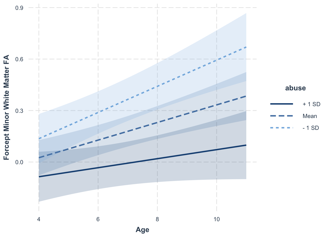
Here we can see some (non-significant) level differences between those who experience low levels of abuse (\(-1\) SD) versus those who experienced mean or high (\(+1\) SD) levels of abuse. However, there are significant slope differences (i.e., the interaction term is significant), such that those who experience lower levels of early childhood abuse also show faster gains in white matter FA. For some additional examples that have both intercept and slope differences, you can consult the help tools for the interactions package here.
In an SEM approach, seeing how to specify a cross-level interaction is easier, although the interaction nature is somewhat more obscured. Implementing the model is trivial, we simply predict both the intercept and slope with our TIC. We again retain the TVC effects for consistency, even though they are not strictly necessary to demonstrate a cross-level interaction.
cross.lcm <- "int =~ 1*ef1 + 1*ef2 + 1*ef3 + 1*ef4
              slp =~ 0*ef1 + 1*ef2 + 2*ef3 + 3*ef4

              ef1 ~ c*dlpfc1
              ef2 ~ c*dlpfc2
              ef3 ~ c*dlpfc3
              ef4 ~ dlpfc4

              int ~ tx
              slp ~ tx"

cross.lcm.fit <- growth(cross.lcm,
                        data = executive.function,
                        estimator = "ML",
                        missing = "FIML")

summary(cross.lcm.fit, fit.measures = FALSE, estimates = TRUE,
        standardize = FALSE, rsquare = FALSE)
## lavaan 0.6.13 ended normally after 33 iterations
##
## Estimator ML
## Optimization method NLMINB
## Number of model parameters 15
## Number of equality constraints 2
##
## Used Total
## Number of observations 296 342
## Number of missing patterns 7
##
## Model Test User Model:
##
## Test statistic 18.561
## Degrees of freedom 21
## P-value (Chi-square) 0.613
##
## Parameter Estimates:
##
## Standard errors Standard
## Information Observed
## Observed information based on Hessian
##
## Latent Variables:
## Estimate Std.Err z-value P(>|z|)
## int =~
## ef1 1.000
## ef2 1.000
## ef3 1.000
## ef4 1.000
## slp =~
## ef1 0.000
## ef2 1.000
## ef3 2.000
## ef4 3.000
##
## Regressions:
## Estimate Std.Err z-value P(>|z|)
## ef1 ~
## dlpfc1 (c) 0.043 0.023 1.918 0.055
## ef2 ~
## dlpfc2 (c) 0.043 0.023 1.918 0.055
## ef3 ~
## dlpfc3 (c) 0.043 0.023 1.918 0.055
## ef4 ~
## dlpfc4 0.095 0.030 3.132 0.002
## int ~
## tx 0.112 0.086 1.294 0.196
## slp ~
## tx 0.000 0.030 0.008 0.994
##
## Covariances:
## Estimate Std.Err z-value P(>|z|)
## .int ~~
## .slp -0.004 0.015 -0.269 0.788
##
## Intercepts:
## Estimate Std.Err z-value P(>|z|)
## .ef1 0.000
## .ef2 0.000
## .ef3 0.000
## .ef4 0.000
## .int 2.390 0.063 37.666 0.000
## .slp 0.033 0.023 1.434 0.151
##
## Variances:
## Estimate Std.Err z-value P(>|z|)
## .ef1 0.219 0.036 6.040 0.000
## .ef2 0.242 0.026 9.125 0.000
## .ef3 0.266 0.029 9.102 0.000
## .ef4 0.137 0.036 3.852 0.000
## .int 0.389 0.049 7.990 0.000
## .slp 0.026 0.008 3.290 0.001Unlike with the MLM, there is no product variable that we enter explicitly into the model. However, we can think about how the slope factor links the TIC and the individual repeated measures. The factor loadings are increasing integers and so the effect of the TIC on each successive repeated measure gets moderated by the numerical value of the factor loading. This serves the same function as an interaction for the SEM approaches.
Time Varying Covariates
While TICs can provide important insights into what factors might contribute to individual differences in the growth trajectories, they fundamentally represent cross-sectional regressions of the latent factors on a set of exogenous variables. However, if we want to test the effects of variables that themselves change over time, we can instead move the TVC model. While TICs predict the growth components (and therefore the repeated measures indirectly; hence cross-level interactions), a TVC directly predicts the individual repeated observations. In this section, we will return to our executive.function dataset. Here we can model the impact of DLPFC activation on executive function scores. As with the TIC model, we will first consider the MLM specification of this approach.
executive.function.long <- executive.function %>%
  pivot_longer(cols = starts_with(c("dlpfc","ef","age")),
               names_to = c(".value", "wave"),
               names_pattern = "(.+)(.)") %>%
  mutate(wave = as.numeric(wave) - 1,
         age = age - min(age, na.rm = TRUE))

tvc.mlm <- lmer(ef ~ 1 + age + dlpfc + (1 + age | id),
                na.action = na.omit,
                REML = TRUE,
                data = executive.function.long,
                control = lmerControl(optimizer = "bobyqa",
                                      optCtrl = list(maxfun = 2e5)))

summary(tvc.mlm, correlation = FALSE)
## Linear mixed model fit by REML. t-tests use Satterthwaite's method [
## lmerModLmerTest]
## Formula: ef ~ 1 + age + dlpfc + (1 + age | id)
## Data: executive.function.long
## Control: lmerControl(optimizer = "bobyqa", optCtrl = list(maxfun = 2e+05))
##
## REML criterion at convergence: 2550
##
## Scaled residuals:
## Min 1Q Median 3Q Max
## -3.2978 -0.4809 0.0377 0.5297 3.1320
##
## Random effects:
## Groups Name Variance Std.Dev. Corr
## id (Intercept) 0.42998 0.6557
## age 0.01877 0.1370 -0.10
## Residual 0.23913 0.4890
## Number of obs: 1241, groups: id, 342
##
## Fixed effects:
## Estimate Std. Error df t value Pr(>|t|)
## (Intercept) 2.371e+00 4.505e-02 3.626e+02 52.623 < 2e-16 ***
## age 4.610e-02 1.516e-02 2.951e+02 3.041 0.00257 **
## dlpfc 5.633e-02 2.062e-02 1.197e+03 2.732 0.00638 **
## ---
## Signif. codes: 0 '***' 0.001 '**' 0.01 '*' 0.05 '.' 0.1 ' ' 1We know have a variable that changes within (i.e., across time) as well as between individuals. Here we have actually somewhat blurred that line but we will talk about how to separate these within- and between-person effects towards the end of this chapter. However, for now we can see that there is a positive effect where more DLPFC activation predicts higher executive function scores. Here this is a purely fixed effect meaning that it holds across all individuals. As with the effect of age; however, we can introduce a random effect of the TVC as well but including it in the random effects structure. This addition allows for the possibility that increasing DLPFC activation has differential effects within different individuals.
rtvc.mlm <- lmer(ef ~ 1 + age + dlpfc + (1 + age + dlpfc | id),
                 na.action = na.omit,
                 REML = TRUE,
                 data = executive.function.long,
                 control = lmerControl(optimizer = "bobyqa",
                                       optCtrl = list(maxfun = 2e5)))

summary(rtvc.mlm, correlation = FALSE)
## Linear mixed model fit by REML. t-tests use Satterthwaite's method [
## lmerModLmerTest]
## Formula: ef ~ 1 + age + dlpfc + (1 + age + dlpfc | id)
## Data: executive.function.long
## Control: lmerControl(optimizer = "bobyqa", optCtrl = list(maxfun = 2e+05))
##
## REML criterion at convergence: 2547.9
##
## Scaled residuals:
## Min 1Q Median 3Q Max
## -3.2787 -0.4949 0.0408 0.5271 3.1584
##
## Random effects:
## Groups Name Variance Std.Dev. Corr
## id (Intercept) 0.443935 0.66628
## age 0.017585 0.13261 -0.13
## dlpfc 0.002587 0.05086 -0.41 0.96
## Residual 0.237147 0.48698
## Number of obs: 1241, groups: id, 342
##
## Fixed effects:
## Estimate Std. Error df t value Pr(>|t|)
## (Intercept) 2.36832 0.04568 307.54702 51.842 < 2e-16 ***
## age 0.04646 0.01498 296.52049 3.102 0.00211 **
## dlpfc 0.05560 0.02092 714.79021 2.658 0.00803 **
## ---
## Signif. codes: 0 '***' 0.001 '**' 0.01 '*' 0.05 '.' 0.1 ' ' 1
## optimizer (bobyqa) convergence code: 0 (OK)
## boundary (singular) fit: see help('isSingular')Here we’ve added \(3\) additional elements in our random effects covariance matrix, one additional variance, and two additional covariances with the effects we had in the prior model. We can see that the correlation between the random slope (age) and DLPFC activation (dlpfc) is quite high. This can lead to estimation issues if this correlation gets too high, and generally reflects redundancy among the random effects.
While the model above already gives us the effect of DLPFC on executive funciton scores above and beyond the growth trajectory, the effects are all contemporaneous. That is, predicting executive function at a given time with DLPFC activation from that same time. A more interesting model is one in which we used activation from one time point to predict executive function at a later time point. While relatively rare, these lagged-effect models really represent a more exciting use of the trouble we went to in order to collect these variables over time. Because of the long format used in MLM, including lagged effects necessitates the creation of a new DLFPC variable with values offset one time point. Fortunately dplyr provides a convenient function to accomplish this data management step. It is; however, important to remember to group by id before creating this new variable so the last value of dlpfc for one person does not shift to the next person’s data rows. In this model, we will drop the random effect of dlpfc for simplicity (and it’s redundancy in the prior model).
executive.function.long <- executive.function.long %>%
  group_by(id) %>%
  mutate(dlpfc.lag = dplyr::lag(dlpfc, 1))

lag.tvc.mlm <- lmer(ef ~ 1 + age + dlpfc + dlpfc.lag + (1 + age | id),
                    na.action = na.omit,
                    REML = TRUE,
                    data = executive.function.long,
                    control = lmerControl(optimizer = "bobyqa",
                                          optCtrl = list(maxfun = 2e5)))

summary(lag.tvc.mlm, correlation = FALSE)
## Linear mixed model fit by REML. t-tests use Satterthwaite's method [
## lmerModLmerTest]
## Formula: ef ~ 1 + age + dlpfc + dlpfc.lag + (1 + age | id)
## Data: executive.function.long
## Control: lmerControl(optimizer = "bobyqa", optCtrl = list(maxfun = 2e+05))
##
## REML criterion at convergence: 1888.8
##
## Scaled residuals:
## Min 1Q Median 3Q Max
## -3.2342 -0.5072 0.0392 0.5511 3.0448
##
## Random effects:
## Groups Name Variance Std.Dev. Corr
## id (Intercept) 0.435953 0.66027
## age 0.001306 0.03614 0.39
## Residual 0.242442 0.49238
## Number of obs: 892, groups: id, 330
##
## Fixed effects:
## Estimate Std. Error df t value Pr(>|t|)
## (Intercept) 2.31372 0.06229 323.33710 37.142 < 2e-16 ***
## age 0.06044 0.02116 281.02897 2.856 0.00461 **
## dlpfc 0.07326 0.02378 814.70968 3.081 0.00213 **
## dlpfc.lag 0.04651 0.02455 823.26058 1.895 0.05850 .
## ---
## Signif. codes: 0 '***' 0.001 '**' 0.01 '*' 0.05 '.' 0.1 ' ' 1Here the effect of the lagged DLPFC variable is non-significant (arbitrary thresholds are arbitrary but live by \(p < .05\), die by \(p < .05\); just be consistent). However, one concerning thing about the lagged MLM model is that we have a reduced sample size compared to the contemporaneous model (contemporaneous: N obs = \(1241\) & N id = \(342\); lagged: N obs = \(892\) & N id = \(330\)). This loss of information is not trivial and comes from two sources. It is helpful to visualize the data frame, which we have done below.
executive.function.long %>% filter(id <= 15 & id >= 10) %>%
  kable(label = NA,
        format = "html",
        digits = 3,
        booktabs = TRUE,
        escape = FALSE,
        caption = "**Executive Function Data with Lagged Variable**",
        align = "c",
        row.names = FALSE) %>%
row_spec(row = 0, align = "c")| id | sex | tx | wave | dlpfc | ef | age | dlpfc.lag |
|---|---|---|---|---|---|---|---|
| 10 | 1 | 1 | 0 | 1.457 | 2.889 | 0.232 | NA |
| 10 | 1 | 1 | 1 | 1.129 | 1.806 | 1.331 | 1.457 |
| 10 | 1 | 1 | 2 | 1.785 | 2.889 | 2.280 | 1.129 |
| 10 | 1 | 1 | 3 | 0.472 | 2.889 | 3.280 | 1.785 |
| 11 | 0 | 1 | 0 | 0.472 | 2.889 | 0.152 | NA |
| 11 | 0 | 1 | 1 | 0.472 | 2.889 | 1.278 | 0.472 |
| 11 | 0 | 1 | 2 | 0.472 | 1.806 | 2.161 | 0.472 |
| 11 | 0 | 1 | 3 | 1.129 | 2.889 | 3.290 | 0.472 |
| 12 | 0 | 1 | 0 | 0.472 | 0.361 | 0.248 | NA |
| 12 | 0 | 1 | 1 | -0.512 | 2.889 | 1.101 | 0.472 |
| 12 | 0 | 1 | 2 | -0.840 | 2.167 | 2.408 | -0.512 |
| 12 | 0 | 1 | 3 | -0.184 | 1.806 | 3.027 | -0.840 |
| 13 | 0 | 1 | 0 | 0.144 | 3.250 | 0.335 | NA |
| 13 | 0 | 1 | 1 | -0.840 | 2.167 | 1.261 | 0.144 |
| 13 | 0 | 1 | 2 | NA | 1.444 | 2.225 | -0.840 |
| 13 | 0 | 1 | 3 | 1.129 | 2.167 | 3.182 | NA |
| 14 | 0 | 0 | 0 | 1.129 | 1.806 | 0.533 | NA |
| 14 | 0 | 0 | 1 | 1.457 | 1.806 | 1.338 | 1.129 |
| 14 | 0 | 0 | 2 | 2.114 | 2.167 | 2.088 | 1.457 |
| 14 | 0 | 0 | 3 | 1.457 | 2.167 | 3.232 | 2.114 |
| 15 | 0 | 1 | 0 | 1.129 | 2.528 | 0.250 | NA |
| 15 | 0 | 1 | 1 | 1.457 | 2.528 | 1.003 | 1.129 |
| 15 | 0 | 1 | 2 | 0.144 | 2.889 | 2.111 | 1.457 |
| 15 | 0 | 1 | 3 | -0.184 | 1.806 | 3.375 | 0.144 |
Note that for every person in our data, we have NA values for the first observation of the dlpfc.lag variable. This is because we could not observe DLPFC activation the time point before we began the study. Because of the conditional likelihood approach we discussed previous as the only option in the MLM, all of these first observation rows are removed from the model. If that wasn’t enough of a bummer, any missing data in the contemporaneous DLPFC variable are shifted to be missing in the lagged version for the next time point, so we lose both time points when we include the contemporaneous and lagged effects (which we should pretty much always do to properly specify the model, so don’t be tempted to only include the lagged effect). We can see this effect for id \(13\) where DLPFC is missing at time \(3\) and so the lagged variable is missing at time \(4\). One potential solution proposed by Dan McNeish is that we replace the NA values for the first observation with a constant, \(0\), so that we don’t lose those time points but they also do not introduce spurious effects. However, we do not want to remove NA values that arise due to true missing data.
executive.function.long[executive.function.long$wave == 0, "dlpfc.lag"] <- 0

lag.tvc.mlm <- lmer(ef ~ 1 + age + dlpfc + dlpfc.lag + (1 + age | id),
                    na.action = na.omit,
                    REML = TRUE,
                    data = executive.function.long,
                    control = lmerControl(optimizer = "bobyqa",
                                          optCtrl = list(maxfun = 2e5)))

summary(lag.tvc.mlm, correlation = FALSE)
## Linear mixed model fit by REML. t-tests use Satterthwaite's method [
## lmerModLmerTest]
## Formula: ef ~ 1 + age + dlpfc + dlpfc.lag + (1 + age | id)
## Data: executive.function.long
## Control: lmerControl(optimizer = "bobyqa", optCtrl = list(maxfun = 2e+05))
##
## REML criterion at convergence: 2523.4
##
## Scaled residuals:
## Min 1Q Median 3Q Max
## -3.3151 -0.4776 0.0375 0.5303 3.0969
##
## Random effects:
## Groups Name Variance Std.Dev. Corr
## id (Intercept) 0.42664 0.6532
## age 0.01684 0.1298 -0.07
## Residual 0.24168 0.4916
## Number of obs: 1224, groups: id, 342
##
## Fixed effects:
## Estimate Std. Error df t value Pr(>|t|)
## (Intercept) 2.367e+00 4.507e-02 3.628e+02 52.516 < 2e-16 ***
## age 3.948e-02 1.620e-02 3.397e+02 2.437 0.01531 *
## dlpfc 5.807e-02 2.085e-02 1.179e+03 2.785 0.00544 **
## dlpfc.lag 4.262e-02 2.186e-02 9.588e+02 1.950 0.05152 .
## ---
## Signif. codes: 0 '***' 0.001 '**' 0.01 '*' 0.05 '.' 0.1 ' ' 1As we can see, the number of observations and id values is much more similar to the contemporaneous effects model. The lag effect is still not significant, but them’s the breaks. Lag effects are often difficult to detect in these kind of longitudinal models due to the relatively long intervals between observations. Relationships simply decay over time and therefore observations spaced out in year or biennial schedules often don’t result in unique lagged effects.
We can also briefly return to the idea of cross-level interactions here. While in the growth model context, we are primarily concerned with cross-level interactions with whatever metric of time we are utilizing in the model, we are not limited to this kind of effect and can moderate the effect of any level 1 TVC with a level 2 TIC. Below might be an example with tx and dlpfc.
cross.mlm <- lmer(ef ~ 1 + age + dlpfc + tx + dlpfc:tx + (1 + age | id),
                  na.action = na.omit,
                  REML = TRUE,
                  data = executive.function.long,
                  control = lmerControl(optimizer = "bobyqa",
                                        optCtrl = list(maxfun = 2e5)))

summary(cross.mlm, correlation = FALSE)
## Linear mixed model fit by REML. t-tests use Satterthwaite's method [
## lmerModLmerTest]
## Formula: ef ~ 1 + age + dlpfc + tx + dlpfc:tx + (1 + age | id)
## Data: executive.function.long
## Control: lmerControl(optimizer = "bobyqa", optCtrl = list(maxfun = 2e+05))
##
## REML criterion at convergence: 2554.8
##
## Scaled residuals:
## Min 1Q Median 3Q Max
## -3.3128 -0.4805 0.0457 0.5191 3.1417
##
## Random effects:
## Groups Name Variance Std.Dev. Corr
## id (Intercept) 0.42661 0.6532
## age 0.01864 0.1365 -0.10
## Residual 0.23955 0.4894
## Number of obs: 1241, groups: id, 342
##
## Fixed effects:
## Estimate Std. Error df t value Pr(>|t|)
## (Intercept) 2.306e+00 6.180e-02 4.211e+02 37.321 <2e-16 ***
## age 4.603e-02 1.516e-02 2.952e+02 3.037 0.0026 **
## dlpfc 5.017e-02 2.990e-02 1.207e+03 1.678 0.0937 .
## tx 1.262e-01 8.229e-02 3.981e+02 1.533 0.1260
## dlpfc:tx 1.256e-02 4.080e-02 1.189e+03 0.308 0.7583
## ---
## Signif. codes: 0 '***' 0.001 '**' 0.01 '*' 0.05 '.' 0.1 ' ' 1interact_plot(model = cross.mlm,
pred = "dlpfc",
modx = "tx",
interval = TRUE,
int.type = "confidence",
x.label = "DLPFC Activation",
y.label = "Executive Function",
modx.labels = c("Treatment", "Control"))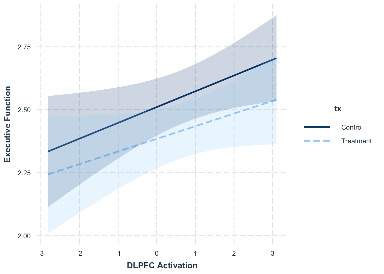
The effects here are not significant, but it is a good principle to keep in mind, especially if fitting these models in a non-growth context.
If we turn to the SEMs, we can re-create many of the models we saw with the MLM (although not exclusively in R), but the SEM does allow for some additional flexibility that may be attractive. Because each measure gets its own column at different time points (i.e., wide format), we need to specify each of the contemporaneous (or lagged) effects individually. However, we will not need to explicitly create a lagged version of the variable. We can see the contemporaneous effect model below. Note that each time-specific regression of ef on dlpfc requires its own line of syntax.
tvc.lcm <- "int =~ 1*ef1 + 1*ef2 + 1*ef3 + 1*ef4
            slp =~ 0*ef1 + 1*ef2 + 2*ef3 + 3*ef4

            ef1 ~ dlpfc1
            ef2 ~ dlpfc2
            ef3 ~ dlpfc3
            ef4 ~ dlpfc4"

tvc.lcm.fit <- growth(tvc.lcm,
                      data = executive.function,
                      estimator = "ML",
                      missing = "FIML")

summary(tvc.lcm.fit, fit.measures = FALSE, estimates = TRUE,
        standardize = FALSE, rsquare = FALSE)
## lavaan 0.6.13 ended normally after 37 iterations
##
## Estimator ML
## Optimization method NLMINB
## Number of model parameters 13
##
## Used Total
## Number of observations 296 342
## Number of missing patterns 7
##
## Model Test User Model:
##
## Test statistic 16.183
## Degrees of freedom 17
## P-value (Chi-square) 0.511
##
## Parameter Estimates:
##
## Standard errors Standard
## Information Observed
## Observed information based on Hessian
##
## Latent Variables:
## Estimate Std.Err z-value P(>|z|)
## int =~
## ef1 1.000
## ef2 1.000
## ef3 1.000
## ef4 1.000
## slp =~
## ef1 0.000
## ef2 1.000
## ef3 2.000
## ef4 3.000
##
## Regressions:
## Estimate Std.Err z-value P(>|z|)
## ef1 ~
## dlpfc1 0.027 0.036 0.773 0.440
## ef2 ~
## dlpfc2 0.051 0.029 1.753 0.080
## ef3 ~
## dlpfc3 0.044 0.031 1.450 0.147
## ef4 ~
## dlpfc4 0.098 0.032 3.080 0.002
##
## Covariances:
## Estimate Std.Err z-value P(>|z|)
## int ~~
## slp -0.003 0.015 -0.229 0.819
##
## Intercepts:
## Estimate Std.Err z-value P(>|z|)
## .ef1 0.000
## .ef2 0.000
## .ef3 0.000
## .ef4 0.000
## int 2.451 0.047 52.040 0.000
## slp 0.030 0.019 1.603 0.109
##
## Variances:
## Estimate Std.Err z-value P(>|z|)
## .ef1 0.220 0.036 6.070 0.000
## .ef2 0.241 0.026 9.119 0.000
## .ef3 0.266 0.029 9.113 0.000
## .ef4 0.138 0.036 3.857 0.000
## int 0.391 0.049 8.001 0.000
## slp 0.026 0.008 3.216 0.001The striking thing here, compared with the MLM results, is that we get \(4\) regression coefficients for the relationship between ef and dlpfc instead of \(1\). These individual time-specific effects are one of the unique strengths of the SEM approaches, and would be essentially impossible to achieve with most MLMs (Mplus is a bit of a potential exception, but that’s because it specifies MLMs more like SEMs), since this is a weird form of nonlinear interaction between the overall TVC effect and time. However, we could also impose simpler functional forms on these regressions. The simplest is to constrain all of them to be equal. This constraint is the one imposed in the MLM, so we should get a single overall TVC effect with this approach. We can see this below.
tvc.lcm <- "int =~ 1*ef1 + 1*ef2 + 1*ef3 + 1*ef4
            slp =~ 0*ef1 + 1*ef2 + 2*ef3 + 3*ef4

            ef1 ~ c*dlpfc1
            ef2 ~ c*dlpfc2
            ef3 ~ c*dlpfc3
            ef4 ~ c*dlpfc4"

tvc.lcm.fit <- growth(tvc.lcm,
                      data = executive.function,
                      estimator = "ML",
                      missing = "FIML")

summary(tvc.lcm.fit, fit.measures = FALSE, estimates = TRUE,
        standardize = FALSE, rsquare = FALSE)
## lavaan 0.6.13 ended normally after 30 iterations
##
## Estimator ML
## Optimization method NLMINB
## Number of model parameters 13
## Number of equality constraints 3
##
## Used Total
## Number of observations 296 342
## Number of missing patterns 7
##
## Model Test User Model:
##
## Test statistic 19.768
## Degrees of freedom 20
## P-value (Chi-square) 0.473
##
## Parameter Estimates:
##
## Standard errors Standard
## Information Observed
## Observed information based on Hessian
##
## Latent Variables:
## Estimate Std.Err z-value P(>|z|)
## int =~
## ef1 1.000
## ef2 1.000
## ef3 1.000
## ef4 1.000
## slp =~
## ef1 0.000
## ef2 1.000
## ef3 2.000
## ef4 3.000
##
## Regressions:
## Estimate Std.Err z-value P(>|z|)
## ef1 ~
## dlpfc1 (c) 0.056 0.021 2.634 0.008
## ef2 ~
## dlpfc2 (c) 0.056 0.021 2.634 0.008
## ef3 ~
## dlpfc3 (c) 0.056 0.021 2.634 0.008
## ef4 ~
## dlpfc4 (c) 0.056 0.021 2.634 0.008
##
## Covariances:
## Estimate Std.Err z-value P(>|z|)
## int ~~
## slp -0.004 0.015 -0.269 0.788
##
## Intercepts:
## Estimate Std.Err z-value P(>|z|)
## .ef1 0.000
## .ef2 0.000
## .ef3 0.000
## .ef4 0.000
## int 2.429 0.045 54.225 0.000
## slp 0.048 0.015 3.124 0.002
##
## Variances:
## Estimate Std.Err z-value P(>|z|)
## .ef1 0.220 0.036 6.067 0.000
## .ef2 0.241 0.026 9.119 0.000
## .ef3 0.266 0.029 9.091 0.000
## .ef4 0.139 0.036 3.896 0.000
## int 0.390 0.049 8.000 0.000
## slp 0.027 0.008 3.308 0.001If we examine the TVC regressions, they are all precisely equal (it should worry us if they are not) and equivalent to the results from the MLM. It is possible through the use of nonlinear constraints to put other functional forms on these regressions. For instance, we could impose a linear constraint so that the regressions increase or decrease over time. We could also impose order constraints where we want the regressions at some time points to be larger than at others. This is where the incredible flexibility of SEM approaches comes out most strongly. The important thing to keep in mind is that this flexibility is also a great way to wander and over-fit our way off a cliff. We need good theoretical justification for our model specification choices and a greater willingness to admit when some features of our model are exploratory to avoid these pitfalls.
One current limitation of implementing SEM TVC models in R is in the inability to specify a random effect of the TVC (to our knowledge). This is possible in Mplus and we have included syntax for that model in the external software downloads.
Finally, the lagged effect model is simple to implement in SEM approaches. We simply include the earlier time point version of our TVC in the regressions for the time-specific outcomes. We won’t need to worry about inducing additional missing data because we never created a lagged version of our TVC.
lag.lcm <- "int =~ 1*ef1 + 1*ef2 + 1*ef3 + 1*ef4
            slp =~ 0*ef1 + 1*ef2 + 2*ef3 + 3*ef4

            ef1 ~ dlpfc1
            ef2 ~ dlpfc2 + dlpfc1
            ef3 ~ dlpfc3 + dlpfc2
            ef4 ~ dlpfc4 + dlpfc3"

lag.lcm.fit <- growth(lag.lcm,
                      data = executive.function,
                      estimator = "ML",
                      missing = "FIML")

summary(lag.lcm.fit, fit.measures = FALSE, estimates = TRUE,
        standardize = FALSE, rsquare = FALSE)
## lavaan 0.6.13 ended normally after 36 iterations
##
## Estimator ML
## Optimization method NLMINB
## Number of model parameters 16
##
## Used Total
## Number of observations 296 342
## Number of missing patterns 7
##
## Model Test User Model:
##
## Test statistic 9.699
## Degrees of freedom 14
## P-value (Chi-square) 0.784
##
## Parameter Estimates:
##
## Standard errors Standard
## Information Observed
## Observed information based on Hessian
##
## Latent Variables:
## Estimate Std.Err z-value P(>|z|)
## int =~
## ef1 1.000
## ef2 1.000
## ef3 1.000
## ef4 1.000
## slp =~
## ef1 0.000
## ef2 1.000
## ef3 2.000
## ef4 3.000
##
## Regressions:
## Estimate Std.Err z-value P(>|z|)
## ef1 ~
## dlpfc1 0.045 0.039 1.154 0.248
## ef2 ~
## dlpfc2 0.067 0.038 1.783 0.075
## dlpfc1 0.008 0.044 0.178 0.859
## ef3 ~
## dlpfc3 0.077 0.039 1.940 0.052
## dlpfc2 0.014 0.037 0.376 0.707
## ef4 ~
## dlpfc4 0.054 0.037 1.455 0.146
## dlpfc3 0.106 0.042 2.507 0.012
##
## Covariances:
## Estimate Std.Err z-value P(>|z|)
## int ~~
## slp -0.005 0.015 -0.333 0.739
##
## Intercepts:
## Estimate Std.Err z-value P(>|z|)
## .ef1 0.000
## .ef2 0.000
## .ef3 0.000
## .ef4 0.000
## int 2.442 0.048 50.832 0.000
## slp 0.020 0.019 1.052 0.293
##
## Variances:
## Estimate Std.Err z-value P(>|z|)
## .ef1 0.220 0.036 6.048 0.000
## .ef2 0.242 0.026 9.143 0.000
## .ef3 0.265 0.029 9.131 0.000
## .ef4 0.133 0.035 3.798 0.000
## int 0.391 0.049 8.007 0.000
## slp 0.026 0.008 3.245 0.001Finally, we could constrain the different types of pathways to be equal within type. While the flexibility of the time-specific effects can be powerful, it can also overwhelm us inferentially. What do we do with the fact that only one of our paths here (ef4 ~ dlpfc3) is significant? Who knows. Constraints can both narrow the number of parameters we are interpreting, but also increase the power to detect an overall effect if one exists because we aggregate over more information.
lag.lcm <- "int =~ 1*ef1 + 1*ef2 + 1*ef3 + 1*ef4
            slp =~ 0*ef1 + 1*ef2 + 2*ef3 + 3*ef4

            ef1 ~ c1*dlpfc1
            ef2 ~ c1*dlpfc2 + c2*dlpfc1
            ef3 ~ c1*dlpfc3 + c2*dlpfc2
            ef4 ~ c1*dlpfc4 + c2*dlpfc3"

lag.lcm.fit <- growth(lag.lcm,
                      data = executive.function,
                      estimator = "ML",
                      missing = "FIML")

summary(lag.lcm.fit, fit.measures = FALSE, estimates = TRUE,
        standardize = FALSE, rsquare = FALSE)
## lavaan 0.6.13 ended normally after 29 iterations
##
## Estimator ML
## Optimization method NLMINB
## Number of model parameters 16
## Number of equality constraints 5
##
## Used Total
## Number of observations 296 342
## Number of missing patterns 7
##
## Model Test User Model:
##
## Test statistic 16.245
## Degrees of freedom 19
## P-value (Chi-square) 0.641
##
## Parameter Estimates:
##
## Standard errors Standard
## Information Observed
## Observed information based on Hessian
##
## Latent Variables:
## Estimate Std.Err z-value P(>|z|)
## int =~
## ef1 1.000
## ef2 1.000
## ef3 1.000
## ef4 1.000
## slp =~
## ef1 0.000
## ef2 1.000
## ef3 2.000
## ef4 3.000
##
## Regressions:
## Estimate Std.Err z-value P(>|z|)
## ef1 ~
## dlpfc1 (c1) 0.057 0.021 2.691 0.007
## ef2 ~
## dlpfc2 (c1) 0.057 0.021 2.691 0.007
## dlpfc1 (c2) 0.042 0.022 1.879 0.060
## ef3 ~
## dlpfc3 (c1) 0.057 0.021 2.691 0.007
## dlpfc2 (c2) 0.042 0.022 1.879 0.060
## ef4 ~
## dlpfc4 (c1) 0.057 0.021 2.691 0.007
## dlpfc3 (c2) 0.042 0.022 1.879 0.060
##
## Covariances:
## Estimate Std.Err z-value P(>|z|)
## int ~~
## slp -0.004 0.015 -0.291 0.771
##
## Intercepts:
## Estimate Std.Err z-value P(>|z|)
## .ef1 0.000
## .ef2 0.000
## .ef3 0.000
## .ef4 0.000
## int 2.423 0.045 53.939 0.000
## slp 0.038 0.016 2.381 0.017
##
## Variances:
## Estimate Std.Err z-value P(>|z|)
## .ef1 0.221 0.036 6.094 0.000
## .ef2 0.243 0.027 9.135 0.000
## .ef3 0.266 0.029 9.115 0.000
## .ef4 0.137 0.035 3.883 0.000
## int 0.389 0.049 7.998 0.000
## slp 0.026 0.008 3.281 0.001This aggregation of course cuts both ways. Now we have no significant lagged effect (although we only had one out of three before so did we really have it to begin with?), but we do have a significant contemporaneous effect where we had no individual one before.
The examples we have included thus far are relatively simple, with a single TVC. Of course all of these models can be expanded to include multiple TVCs, and potentially interactions if we have the sample size to support them.
Multivariate Models
Those paying close attention (and at this point all the kudos to you) might have been a bit perturbed by the fact that in our Canonical chapter, we fit a growth model to the dlpfc variable, but here we have used it as our TVC. This is indeed of great concern and something we should always be thinking about when including a repeated measure as a TVC. The standard TVC model assumes that there are no systematic changes in the covariate across time. The values obviously change, but not systematically. Rather, the traditional TVC model is well suited for covariates that fluctuates from time point to time point. Weather over short intervals is often a canonical example in more-intensive applications, but we can think also the time of day that testing occurs as one that might be of interest for our purposes. From our earlier model fitting, we know that our dlpfc TVC does not meet this criteria. This is an issue because we essentially have an unmodeled age effect on the TVC, which will introduce bias into our model results.
The other issue is that of true exogeneity. Do we really believe that the causal effect in our model only runs from DLPFC activation to executive function, and that there are no reciprocal relationships over time? With something like the weather this is totally plausible; however, with our data this assumption seems unlikely to hold. As such, we might wish to treat both ef and dlpfc as outcomes in a multivariate model. This will involve some difficulty in the MLM, but will be a completely natural extension of the SEM. We will flip our usual order of considering the MLM first and demonstrate the SEM specifications so it’s easier to see where we will run into difficulty with the MLMs. We will first re-fit the TVC model we ended with earlier
tvc.lcm <- "int =~ 1*ef1 + 1*ef2 + 1*ef3 + 1*ef4
            slp =~ 0*ef1 + 1*ef2 + 2*ef3 + 3*ef4

            ef1 ~ c*dlpfc1
            ef2 ~ c*dlpfc2
            ef3 ~ c*dlpfc3
            ef4 ~ c*dlpfc4"

tvc.lcm.fit <- growth(tvc.lcm,
                      data = executive.function,
                      estimator = "ML",
                      missing = "FIML")

summary(tvc.lcm.fit, fit.measures = FALSE, estimates = TRUE,
        standardize = FALSE, rsquare = FALSE)
## lavaan 0.6.13 ended normally after 30 iterations
##
## Estimator ML
## Optimization method NLMINB
## Number of model parameters 13
## Number of equality constraints 3
##
## Used Total
## Number of observations 296 342
## Number of missing patterns 7
##
## Model Test User Model:
##
## Test statistic 19.768
## Degrees of freedom 20
## P-value (Chi-square) 0.473
##
## Parameter Estimates:
##
## Standard errors Standard
## Information Observed
## Observed information based on Hessian
##
## Latent Variables:
## Estimate Std.Err z-value P(>|z|)
## int =~
## ef1 1.000
## ef2 1.000
## ef3 1.000
## ef4 1.000
## slp =~
## ef1 0.000
## ef2 1.000
## ef3 2.000
## ef4 3.000
##
## Regressions:
## Estimate Std.Err z-value P(>|z|)
## ef1 ~
## dlpfc1 (c) 0.056 0.021 2.634 0.008
## ef2 ~
## dlpfc2 (c) 0.056 0.021 2.634 0.008
## ef3 ~
## dlpfc3 (c) 0.056 0.021 2.634 0.008
## ef4 ~
## dlpfc4 (c) 0.056 0.021 2.634 0.008
##
## Covariances:
## Estimate Std.Err z-value P(>|z|)
## int ~~
## slp -0.004 0.015 -0.269 0.788
##
## Intercepts:
## Estimate Std.Err z-value P(>|z|)
## .ef1 0.000
## .ef2 0.000
## .ef3 0.000
## .ef4 0.000
## int 2.429 0.045 54.225 0.000
## slp 0.048 0.015 3.124 0.002
##
## Variances:
## Estimate Std.Err z-value P(>|z|)
## .ef1 0.220 0.036 6.067 0.000
## .ef2 0.241 0.026 9.119 0.000
## .ef3 0.266 0.029 9.091 0.000
## .ef4 0.139 0.036 3.896 0.000
## int 0.390 0.049 8.000 0.000
## slp 0.027 0.008 3.308 0.001To transform this model into a multivariate version, we need to estimate an intercept and slope for both the ef and the dlpfc variables. One thing to note is that we should be explicit about including the correlations between the growth factors within- and across-construct, as well as cross-construct, time-specific covariances between the individual repeated measures. These time-specific residuals are often necessary and help account for unmeasured common causes that might induce correlations among the repeated measures above-and-beyond the growth factors themselves. We can do all the usual things with these residual covariances, including testing equality constraints or even constraining them to zero and assess their impact on model fit through likelihood ratio tests. For now we will estimate unique relationships, as that is the default in SEM approaches.
multivar.lcm <- "
                 # Growth Factors for EF
                 int.ef =~ 1*ef1 + 1*ef2 + 1*ef3 + 1*ef4
                 slp.ef =~ 0*ef1 + 1*ef2 + 2*ef3 + 3*ef4

                 # Growth Factors for DLPFC
                 int.dlpfc =~ 1*dlpfc1 + 1*dlpfc2 + 1*dlpfc3 + 1*dlpfc4
                 slp.dlpfc =~ 0*dlpfc1 + 1*dlpfc2 + 2*dlpfc3 + 3*dlpfc4

                 # Factor Covariances
                 int.ef ~~ slp.ef + int.dlpfc + slp.dlpfc
                 slp.ef ~~ int.dlpfc + slp.dlpfc
                 int.dlpfc ~~ slp.dlpfc

                 # Time-Specific Residual Covariance
                 ef1 ~~ dlpfc1
                 ef2 ~~ dlpfc2
                 ef3 ~~ dlpfc3
                 ef4 ~~ dlpfc4"

multivar.lcm.fit <- growth(multivar.lcm,
                           data = executive.function,
                           estimator = "ML",
                           missing = "FIML")

summary(multivar.lcm.fit, fit.measures = FALSE, estimates = TRUE,
        standardize = FALSE, rsquare = FALSE)
## lavaan 0.6.13 ended normally after 50 iterations
##
## Estimator ML
## Optimization method NLMINB
## Number of model parameters 26
##
## Number of observations 342
## Number of missing patterns 28
##
## Model Test User Model:
##
## Test statistic 11.574
## Degrees of freedom 18
## P-value (Chi-square) 0.868
##
## Parameter Estimates:
##
## Standard errors Standard
## Information Observed
## Observed information based on Hessian
##
## Latent Variables:
## Estimate Std.Err z-value P(>|z|)
## int.ef =~
## ef1 1.000
## ef2 1.000
## ef3 1.000
## ef4 1.000
## slp.ef =~
## ef1 0.000
## ef2 1.000
## ef3 2.000
## ef4 3.000
## int.dlpfc =~
## dlpfc1 1.000
## dlpfc2 1.000
## dlpfc3 1.000
## dlpfc4 1.000
## slp.dlpfc =~
## dlpfc1 0.000
## dlpfc2 1.000
## dlpfc3 2.000
## dlpfc4 3.000
##
## Covariances:
## Estimate Std.Err z-value P(>|z|)
## int.ef ~~
## slp.ef -0.010 0.016 -0.634 0.526
## int.dlpfc 0.084 0.046 1.823 0.068
## slp.dlpfc -0.022 0.019 -1.159 0.247
## slp.ef ~~
## int.dlpfc 0.011 0.017 0.647 0.518
## slp.dlpfc 0.011 0.008 1.319 0.187
## int.dlpfc ~~
## slp.dlpfc -0.125 0.031 -4.072 0.000
## .ef1 ~~
## .dlpfc1 -0.037 0.035 -1.066 0.286
## .ef2 ~~
## .dlpfc2 0.048 0.027 1.738 0.082
## .ef3 ~~
## .dlpfc3 0.023 0.029 0.781 0.435
## .ef4 ~~
## .dlpfc4 -0.013 0.037 -0.348 0.728
##
## Intercepts:
## Estimate Std.Err z-value P(>|z|)
## .ef1 0.000
## .ef2 0.000
## .ef3 0.000
## .ef4 0.000
## .dlpfc1 0.000
## .dlpfc2 0.000
## .dlpfc3 0.000
## .dlpfc4 0.000
## int.ef 2.407 0.042 57.447 0.000
## slp.ef 0.059 0.015 3.921 0.000
## int.dlpfc 0.545 0.053 10.212 0.000
## slp.dlpfc 0.120 0.021 5.696 0.000
##
## Variances:
## Estimate Std.Err z-value P(>|z|)
## .ef1 0.236 0.038 6.250 0.000
## .ef2 0.262 0.027 9.569 0.000
## .ef3 0.263 0.028 9.329 0.000
## .ef4 0.123 0.034 3.615 0.000
## .dlpfc1 0.235 0.063 3.733 0.000
## .dlpfc2 0.566 0.055 10.268 0.000
## .dlpfc3 0.577 0.057 10.110 0.000
## .dlpfc4 0.399 0.074 5.389 0.000
## int.ef 0.425 0.050 8.485 0.000
## slp.ef 0.030 0.008 3.675 0.000
## int.dlpfc 0.775 0.086 9.020 0.000
## slp.dlpfc 0.081 0.016 5.134 0.000This model is quite simple for a SEM approach, and we can examine how different constructs travel together over time by examining the inter-relations among the growth factors. However, this is ultimately cross-sectional correlations because there is no temporal order at the latent level, either between intercepts and slope or between factors of different constructs. If we want to examine cross-lagged relationships among the repeated measures themselves (ala the standard cross-lag panel model we won’t consider here for numerous reasons), we might wish to introduce regression relationships among the repeated measures.
There are several ways to specify these regression among the repeated measures in a multivariate growth model; however, we will focus on what is known as the random-intercept cross-lag panel model (RI-CLPM) and it’s generalization in the latent curve model with structured residuals (LCM-SR). For an overview of potential alternatives, see Usami & Hamaker, 2019. We retain the time-specific residual covariances, but now we include regression coefficients between the residuals of the repeated measures (hence “structured residuals”). Note that for the RI-CLPM, we remove the slope factors. In the LCM-SR, we can include any combination of latent growth factors, so that will be the term we will use to reference this general type of model, with the RI-CLPM being a special case.
riclpm <- "
          # Random Intercept for EF
          int.ef =~ 1*ef1 + 1*ef2 + 1*ef3 + 1*ef4

          # Random Intercept for DLPFC
          int.dlpfc =~ 1*dlpfc1 + 1*dlpfc2 + 1*dlpfc3 + 1*dlpfc4

          # Factor Covariances
          int.ef ~~ int.dlpfc

          # Time-Specific Residual Covariance
          ef1 ~~ dlpfc1
          ef2 ~~ dlpfc2
          ef3 ~~ dlpfc3
          ef4 ~~ dlpfc4

          # Autoregressive and Cross-Regressive Effects
          ef2 ~ ef1 + dlpfc1
          ef3 ~ ef2 + dlpfc2
          ef4 ~ ef3 + dlpfc3
          dlpfc2 ~ dlpfc1 + ef1
          dlpfc3 ~ dlpfc2 + ef2
          dlpfc4 ~ dlpfc3 + ef3"

riclpm.fit <- growth(riclpm,
                     data = executive.function,
                     estimator = "ML",
                     missing = "FIML")

summary(riclpm.fit, fit.measures = FALSE, estimates = TRUE,
        standardize = FALSE, rsquare = FALSE)
## lavaan 0.6.13 ended normally after 44 iterations
##
## Estimator ML
## Optimization method NLMINB
## Number of model parameters 29
##
## Number of observations 342
## Number of missing patterns 28
##
## Model Test User Model:
##
## Test statistic 30.269
## Degrees of freedom 15
## P-value (Chi-square) 0.011
##
## Parameter Estimates:
##
## Standard errors Standard
## Information Observed
## Observed information based on Hessian
##
## Latent Variables:
## Estimate Std.Err z-value P(>|z|)
## int.ef =~
## ef1 1.000
## ef2 1.000
## ef3 1.000
## ef4 1.000
## int.dlpfc =~
## dlpfc1 1.000
## dlpfc2 1.000
## dlpfc3 1.000
## dlpfc4 1.000
##
## Regressions:
## Estimate Std.Err z-value P(>|z|)
## ef2 ~
## ef1 0.027 0.018 1.472 0.141
## dlpfc1 0.022 0.037 0.605 0.545
## ef3 ~
## ef2 0.034 0.019 1.792 0.073
## dlpfc2 0.034 0.035 0.971 0.332
## ef4 ~
## ef3 0.065 0.019 3.490 0.000
## dlpfc3 0.087 0.034 2.579 0.010
## dlpfc2 ~
## dlpfc1 0.291 0.065 4.481 0.000
## ef1 -0.001 0.027 -0.042 0.966
## dlpfc3 ~
## dlpfc2 0.131 0.063 2.083 0.037
## ef2 0.052 0.029 1.771 0.077
## dlpfc4 ~
## dlpfc3 0.175 0.061 2.886 0.004
## ef3 0.081 0.029 2.795 0.005
##
## Covariances:
## Estimate Std.Err z-value P(>|z|)
## int.ef ~~
## int.dlpfc 0.030 0.032 0.959 0.338
## .ef1 ~~
## .dlpfc1 -0.008 0.033 -0.243 0.808
## .ef2 ~~
## .dlpfc2 0.050 0.029 1.711 0.087
## .ef3 ~~
## .dlpfc3 0.060 0.033 1.827 0.068
## .ef4 ~~
## .dlpfc4 0.022 0.030 0.724 0.469
##
## Intercepts:
## Estimate Std.Err z-value P(>|z|)
## .ef1 0.000
## .ef2 0.000
## .ef3 0.000
## .ef4 0.000
## .dlpfc1 0.000
## .dlpfc2 0.000
## .dlpfc3 0.000
## .dlpfc4 0.000
## int.ef 2.390 0.046 52.341 0.000
## int.dlpfc 0.546 0.052 10.501 0.000
##
## Variances:
## Estimate Std.Err z-value P(>|z|)
## .ef1 0.313 0.032 9.656 0.000
## .ef2 0.262 0.028 9.267 0.000
## .ef3 0.280 0.030 9.445 0.000
## .ef4 0.229 0.026 8.773 0.000
## .dlpfc1 0.627 0.069 9.120 0.000
## .dlpfc2 0.568 0.060 9.507 0.000
## .dlpfc3 0.669 0.069 9.660 0.000
## .dlpfc4 0.639 0.062 10.310 0.000
## int.ef 0.412 0.040 10.263 0.000
## int.dlpfc 0.352 0.063 5.551 0.000With the LCM-SR, we simply add back the slope factors for each of our constructs. Note that in practice, we do not need to specify the same type of trajectory for each variable. It’s entirely possible that one variable might follow a linear and the other a quadratic. Indeed one construct might only need a random intercept (we will see this later); we can mix and match as we please.
lcmsr <- "
         # Growth Factors for EF
         int.ef =~ 1*ef1 + 1*ef2 + 1*ef3 + 1*ef4
         slp.ef =~ 0*ef1 + 1*ef2 + 2*ef3 + 3*ef4

         # Growth Factors for DLPFC
         int.dlpfc =~ 1*dlpfc1 + 1*dlpfc2 + 1*dlpfc3 + 1*dlpfc4
         slp.dlpfc =~ 0*dlpfc1 + 1*dlpfc2 + 2*dlpfc3 + 3*dlpfc4

         # Factor Covariances
         int.ef ~~ slp.ef + int.dlpfc + slp.dlpfc
         slp.ef ~~ int.dlpfc + slp.dlpfc
         int.dlpfc ~~ slp.dlpfc

         # Time-Specific Residual Covariance
         ef1 ~~ dlpfc1
         ef2 ~~ dlpfc2
         ef3 ~~ dlpfc3
         ef4 ~~ dlpfc4

         # Autoregressive and Cross-Regressive Effects
         ef2 ~ ef1 + dlpfc1
         ef3 ~ ef2 + dlpfc2
         ef4 ~ ef3 + dlpfc3
         dlpfc2 ~ dlpfc1 + ef1
         dlpfc3 ~ dlpfc2 + ef2
         dlpfc4 ~ dlpfc3 + ef3"

lcmsr.fit <- growth(lcmsr,
                    data = executive.function,
                    estimator = "ML",
                    missing = "FIML")

summary(lcmsr.fit, fit.measures = FALSE, estimates = TRUE,
        standardize = FALSE, rsquare = FALSE)
## lavaan 0.6.13 ended normally after 72 iterations
##
## Estimator ML
## Optimization method NLMINB
## Number of model parameters 38
##
## Number of observations 342
## Number of missing patterns 28
##
## Model Test User Model:
##
## Test statistic 1.299
## Degrees of freedom 6
## P-value (Chi-square) 0.972
##
## Parameter Estimates:
##
## Standard errors Standard
## Information Observed
## Observed information based on Hessian
##
## Latent Variables:
## Estimate Std.Err z-value P(>|z|)
## int.ef =~
## ef1 1.000
## ef2 1.000
## ef3 1.000
## ef4 1.000
## slp.ef =~
## ef1 0.000
## ef2 1.000
## ef3 2.000
## ef4 3.000
## int.dlpfc =~
## dlpfc1 1.000
## dlpfc2 1.000
## dlpfc3 1.000
## dlpfc4 1.000
## slp.dlpfc =~
## dlpfc1 0.000
## dlpfc2 1.000
## dlpfc3 2.000
## dlpfc4 3.000
##
## Regressions:
## Estimate Std.Err z-value P(>|z|)
## ef2 ~
## ef1 0.022 0.048 0.463 0.643
## dlpfc1 0.031 0.047 0.664 0.507
## ef3 ~
## ef2 0.035 0.088 0.402 0.688
## dlpfc2 0.074 0.044 1.702 0.089
## ef4 ~
## ef3 0.052 0.133 0.390 0.697
## dlpfc3 0.191 0.076 2.522 0.012
## dlpfc2 ~
## dlpfc1 0.030 0.087 0.346 0.729
## ef1 0.091 0.054 1.699 0.089
## dlpfc3 ~
## dlpfc2 0.006 0.076 0.077 0.939
## ef2 0.163 0.096 1.702 0.089
## dlpfc4 ~
## dlpfc3 -0.062 0.155 -0.403 0.687
## ef3 0.274 0.145 1.887 0.059
##
## Covariances:
## Estimate Std.Err z-value P(>|z|)
## int.ef ~~
## slp.ef -0.020 0.019 -1.030 0.303
## int.dlpfc 0.069 0.057 1.202 0.229
## slp.dlpfc -0.046 0.026 -1.752 0.080
## slp.ef ~~
## int.dlpfc -0.016 0.022 -0.731 0.465
## slp.dlpfc -0.009 0.013 -0.675 0.500
## int.dlpfc ~~
## slp.dlpfc -0.115 0.046 -2.504 0.012
## .ef1 ~~
## .dlpfc1 -0.013 0.046 -0.287 0.774
## .ef2 ~~
## .dlpfc2 0.059 0.029 2.044 0.041
## .ef3 ~~
## .dlpfc3 0.113 0.047 2.392 0.017
## .ef4 ~~
## .dlpfc4 0.059 0.056 1.057 0.291
##
## Intercepts:
## Estimate Std.Err z-value P(>|z|)
## .ef1 0.000
## .ef2 0.000
## .ef3 0.000
## .ef4 0.000
## .dlpfc1 0.000
## .dlpfc2 0.000
## .dlpfc3 0.000
## .dlpfc4 0.000
## int.ef 2.421 0.044 54.641 0.000
## slp.ef -0.033 0.112 -0.298 0.765
## int.dlpfc 0.539 0.054 9.985 0.000
## slp.dlpfc -0.089 0.124 -0.715 0.475
##
## Variances:
## Estimate Std.Err z-value P(>|z|)
## .ef1 0.238 0.045 5.345 0.000
## .ef2 0.268 0.030 8.961 0.000
## .ef3 0.282 0.045 6.270 0.000
## .ef4 0.144 0.051 2.815 0.005
## .dlpfc1 0.262 0.106 2.466 0.014
## .dlpfc2 0.559 0.058 9.605 0.000
## .dlpfc3 0.557 0.099 5.614 0.000
## .dlpfc4 0.409 0.103 3.980 0.000
## int.ef 0.424 0.056 7.640 0.000
## slp.ef 0.025 0.013 1.931 0.054
## int.dlpfc 0.736 0.125 5.898 0.000
## slp.dlpfc 0.086 0.027 3.252 0.001For all the reasons we have discussed so far (and common practice in CLPMs more generally), it is common to test equality constraints on the auto- and cross-regressive effects in these models. We can see an example of this below.
lcmsr <- "
         # Growth Factors for EF
         int.ef =~ 1*ef1 + 1*ef2 + 1*ef3 + 1*ef4
         slp.ef =~ 0*ef1 + 1*ef2 + 2*ef3 + 3*ef4

         # Growth Factors for DLPFC
         int.dlpfc =~ 1*dlpfc1 + 1*dlpfc2 + 1*dlpfc3 + 1*dlpfc4
         slp.dlpfc =~ 0*dlpfc1 + 1*dlpfc2 + 2*dlpfc3 + 3*dlpfc4

         # Factor Covariances
         int.ef ~~ slp.ef + int.dlpfc + slp.dlpfc
         slp.ef ~~ int.dlpfc + slp.dlpfc
         int.dlpfc ~~ slp.dlpfc

         # Time-Specific Residual Covariance
         ef1 ~~ dlpfc1
         ef2 ~~ dlpfc2
         ef3 ~~ dlpfc3
         ef4 ~~ dlpfc4

         # Autoregressive and Cross-Regressive Effects
         ef2 ~ c1*ef1 + c3*dlpfc1
         ef3 ~ c1*ef2 + c3*dlpfc2
         ef4 ~ c1*ef3 + c3*dlpfc3
         dlpfc2 ~ c2*dlpfc1 + c4*ef1
         dlpfc3 ~ c2*dlpfc2 + c4*ef2
         dlpfc4 ~ c2*dlpfc3 + c4*ef3"

lcmsr.fit <- growth(lcmsr,
                    data = executive.function,
                    estimator = "ML",
                    missing = "FIML")

summary(lcmsr.fit, fit.measures = FALSE, estimates = TRUE,
        standardize = FALSE, rsquare = FALSE)
## lavaan 0.6.13 ended normally after 57 iterations
##
## Estimator ML
## Optimization method NLMINB
## Number of model parameters 38
## Number of equality constraints 8
##
## Number of observations 342
## Number of missing patterns 28
##
## Model Test User Model:
##
## Test statistic 9.555
## Degrees of freedom 14
## P-value (Chi-square) 0.794
##
## Parameter Estimates:
##
## Standard errors Standard
## Information Observed
## Observed information based on Hessian
##
## Latent Variables:
## Estimate Std.Err z-value P(>|z|)
## int.ef =~
## ef1 1.000
## ef2 1.000
## ef3 1.000
## ef4 1.000
## slp.ef =~
## ef1 0.000
## ef2 1.000
## ef3 2.000
## ef4 3.000
## int.dlpfc =~
## dlpfc1 1.000
## dlpfc2 1.000
## dlpfc3 1.000
## dlpfc4 1.000
## slp.dlpfc =~
## dlpfc1 0.000
## dlpfc2 1.000
## dlpfc3 2.000
## dlpfc4 3.000
##
## Regressions:
## Estimate Std.Err z-value P(>|z|)
## ef2 ~
## ef1 (c1) -0.020 0.020 -1.010 0.312
## dlpfc1 (c3) 0.030 0.030 0.979 0.328
## ef3 ~
## ef2 (c1) -0.020 0.020 -1.010 0.312
## dlpfc2 (c3) 0.030 0.030 0.979 0.328
## ef4 ~
## ef3 (c1) -0.020 0.020 -1.010 0.312
## dlpfc3 (c3) 0.030 0.030 0.979 0.328
## dlpfc2 ~
## dlpfc1 (c2) 0.026 0.061 0.419 0.675
## ef1 (c4) 0.014 0.028 0.497 0.619
## dlpfc3 ~
## dlpfc2 (c2) 0.026 0.061 0.419 0.675
## ef2 (c4) 0.014 0.028 0.497 0.619
## dlpfc4 ~
## dlpfc3 (c2) 0.026 0.061 0.419 0.675
## ef3 (c4) 0.014 0.028 0.497 0.619
##
## Covariances:
## Estimate Std.Err z-value P(>|z|)
## int.ef ~~
## slp.ef -0.012 0.016 -0.774 0.439
## int.dlpfc 0.062 0.051 1.204 0.229
## slp.dlpfc -0.016 0.021 -0.801 0.423
## slp.ef ~~
## int.dlpfc 0.013 0.017 0.739 0.460
## slp.dlpfc 0.005 0.009 0.584 0.559
## int.dlpfc ~~
## slp.dlpfc -0.124 0.032 -3.849 0.000
## .ef1 ~~
## .dlpfc1 -0.018 0.039 -0.447 0.655
## .ef2 ~~
## .dlpfc2 0.049 0.027 1.775 0.076
## .ef3 ~~
## .dlpfc3 0.031 0.030 1.020 0.308
## .ef4 ~~
## .dlpfc4 0.001 0.039 0.018 0.985
##
## Intercepts:
## Estimate Std.Err z-value P(>|z|)
## .ef1 0.000
## .ef2 0.000
## .ef3 0.000
## .ef4 0.000
## .dlpfc1 0.000
## .dlpfc2 0.000
## .dlpfc3 0.000
## .dlpfc4 0.000
## int.ef 2.419 0.044 54.605 0.000
## slp.ef 0.066 0.021 3.159 0.002
## int.dlpfc 0.536 0.054 9.901 0.000
## slp.dlpfc 0.102 0.032 3.178 0.001
##
## Variances:
## Estimate Std.Err z-value P(>|z|)
## .ef1 0.224 0.039 5.746 0.000
## .ef2 0.261 0.027 9.571 0.000
## .ef3 0.258 0.028 9.191 0.000
## .ef4 0.115 0.035 3.342 0.001
## .dlpfc1 0.253 0.085 2.969 0.003
## .dlpfc2 0.566 0.055 10.214 0.000
## .dlpfc3 0.592 0.064 9.304 0.000
## .dlpfc4 0.413 0.088 4.677 0.000
## int.ef 0.439 0.053 8.349 0.000
## slp.ef 0.032 0.009 3.736 0.000
## int.dlpfc 0.754 0.106 7.134 0.000
## slp.dlpfc 0.077 0.021 3.668 0.000As always, we can extend this model in a number of ways that we won’t go into here for sake of time (ha ha ha you may say to yourself). While uncommon, we could impose functions on the cross-regressive paths, add additional outcome variables, and include both TIC and (true) TVCs to this model. The limitations are as always, proper theoretical models for that complexity, and sufficient data to estimate all of these effects uniquely.
Multivariate LCSMs have some additional peculiarities that we will explore since they diverge somewhat from the LCM we have mostly focused on. However, as with all SEMs, the problem is much more keeping track of the parameter syntax than it is an inability to estimate certain effects. The main point of divergence between the LCM and LCSM is the inclusion of proportional parameters in the multivariate model. Because of this, we will dive straight into that model instead of building up in the way we did with the LCM. Below we can see the syntax for this multivariate dual-change LCSM.
multivar.dualchange <- "
        # Define Phantom Variables (p = phantom)
        pef1 =~ 1*ef1; ef1 ~ 0; ef1 ~~ ef1; pef1 ~~ 0*pef1
        pef2 =~ 1*ef2; ef2 ~ 0; ef2 ~~ ef2; pef2 ~~ 0*pef2
        pef3 =~ 1*ef3; ef3 ~ 0; ef3 ~~ ef3; pef3 ~~ 0*pef3
        pef4 =~ 1*ef4; ef4 ~ 0; ef4 ~~ ef4; pef4 ~~ 0*pef4

        pdlpfc1 =~ 1*dlpfc1; dlpfc1 ~ 0; dlpfc1 ~~ dlpfc1; pdlpfc1 ~~ 0*pdlpfc1
        pdlpfc2 =~ 1*dlpfc2; dlpfc2 ~ 0; dlpfc2 ~~ dlpfc2; pdlpfc2 ~~ 0*pdlpfc2
        pdlpfc3 =~ 1*dlpfc3; dlpfc3 ~ 0; dlpfc3 ~~ dlpfc3; pdlpfc3 ~~ 0*pdlpfc3
        pdlpfc4 =~ 1*dlpfc4; dlpfc4 ~ 0; dlpfc4 ~~ dlpfc4; pdlpfc4 ~~ 0*pdlpfc4

        # Regressions Between Adjacent Observations
        pef2 ~ 1*pef1
        pef3 ~ 1*pef2
        pef4 ~ 1*pef3

        pdlpfc2 ~ 1*pdlpfc1
        pdlpfc3 ~ 1*pdlpfc2
        pdlpfc4 ~ 1*pdlpfc3

        # Define Change Latent Variables (d)
        def21 =~ 1*pef2; def21 ~~ 0*def21
        def32 =~ 1*pef3; def32 ~~ 0*def32
        def43 =~ 1*pef4; def43 ~~ 0*def43

        ddlpfc21 =~ 1*pdlpfc2; ddlpfc21 ~~ 0*ddlpfc21
        ddlpfc32 =~ 1*pdlpfc3; ddlpfc32 ~~ 0*ddlpfc32
        ddlpfc43 =~ 1*pdlpfc4; ddlpfc43 ~~ 0*ddlpfc43

        # Define Proportional Change Regressions (beta = equality constraint)
        def21 ~ beta1*pef1 + beta3*pdlpfc1
        def32 ~ beta1*pef2 + beta3*pdlpfc2
        def43 ~ beta1*pef3 + beta3*pdlpfc3

        ddlpfc21 ~ beta2*pdlpfc1 + beta4*pef1
        ddlpfc32 ~ beta2*pdlpfc2 + beta4*pef2
        ddlpfc43 ~ beta2*pdlpfc3 + beta4*pef3

        # Define Intercept and Slope
        int.ef =~ 1*pef1
        slp.ef =~ 1*def21 + 1*def32 + 1*def43
        int.ef ~ 1; int.ef ~~ int.ef
        slp.ef ~ 1; slp.ef ~~ slp.ef
        int.ef ~~ slp.ef

        int.dlpfc =~ 1*pdlpfc1
        slp.dlpfc =~ 1*ddlpfc21 + 1*ddlpfc32 + 1*ddlpfc43
        int.dlpfc ~ 1; int.dlpfc ~~ int.dlpfc
        slp.dlpfc ~ 1; slp.dlpfc ~~ slp.dlpfc
        int.dlpfc ~~ slp.dlpfc

        # Cross-Construct Covariances
        int.ef ~~ int.dlpfc + slp.dlpfc
        slp.ef ~~ int.dlpfc + slp.dlpfc
"

multivar.dualchange <- sem(multivar.dualchange,
                           data = executive.function,
                           estimator = "ML",
                           missing = "FIML")

summary(multivar.dualchange, fit.measures = FALSE, estimates = TRUE,
        standardize = FALSE, rsquare = FALSE)
## lavaan 0.6.13 ended normally after 122 iterations
##
## Estimator ML
## Optimization method NLMINB
## Number of model parameters 34
## Number of equality constraints 8
##
## Number of observations 342
## Number of missing patterns 28
##
## Model Test User Model:
##
## Test statistic 14.490
## Degrees of freedom 18
## P-value (Chi-square) 0.697
##
## Parameter Estimates:
##
## Standard errors Standard
## Information Observed
## Observed information based on Hessian
##
## Latent Variables:
## Estimate Std.Err z-value P(>|z|)
## pef1 =~
## ef1 1.000
## pef2 =~
## ef2 1.000
## pef3 =~
## ef3 1.000
## pef4 =~
## ef4 1.000
## pdlpfc1 =~
## dlpfc1 1.000
## pdlpfc2 =~
## dlpfc2 1.000
## pdlpfc3 =~
## dlpfc3 1.000
## pdlpfc4 =~
## dlpfc4 1.000
## def21 =~
## pef2 1.000
## def32 =~
## pef3 1.000
## def43 =~
## pef4 1.000
## ddlpfc21 =~
## pdlpfc2 1.000
## ddlpfc32 =~
## pdlpfc3 1.000
## ddlpfc43 =~
## pdlpfc4 1.000
## int.ef =~
## pef1 1.000
## slp.ef =~
## def21 1.000
## def32 1.000
## def43 1.000
## int.dlpfc =~
## pdlpfc1 1.000
## slp.dlpfc =~
## ddlpfc21 1.000
## ddlpfc32 1.000
## ddlpfc43 1.000
##
## Regressions:
## Estimate Std.Err z-value P(>|z|)
## pef2 ~
## pef1 1.000
## pef3 ~
## pef2 1.000
## pef4 ~
## pef3 1.000
## pdlpfc2 ~
## pdlpfc1 1.000
## pdlpfc3 ~
## pdlpfc2 1.000
## pdlpfc4 ~
## pdlpfc3 1.000
## def21 ~
## pef1 (bet1) 0.249 0.596 0.418 0.676
## pdlpfc1 (bet3) 0.069 0.155 0.448 0.654
## def32 ~
## pef2 (bet1) 0.249 0.596 0.418 0.676
## pdlpfc2 (bet3) 0.069 0.155 0.448 0.654
## def43 ~
## pef3 (bet1) 0.249 0.596 0.418 0.676
## pdlpfc3 (bet3) 0.069 0.155 0.448 0.654
## ddlpfc21 ~
## pdlpfc1 (bet2) -0.077 0.379 -0.204 0.839
## pef1 (bet4) 0.067 0.425 0.157 0.875
## ddlpfc32 ~
## pdlpfc2 (bet2) -0.077 0.379 -0.204 0.839
## pef2 (bet4) 0.067 0.425 0.157 0.875
## ddlpfc43 ~
## pdlpfc3 (bet2) -0.077 0.379 -0.204 0.839
## pef3 (bet4) 0.067 0.425 0.157 0.875
##
## Covariances:
## Estimate Std.Err z-value P(>|z|)
## int.ef ~~
## slp.ef -0.118 0.244 -0.483 0.629
## int.dlpfc ~~
## slp.dlpfc -0.085 0.197 -0.430 0.667
## int.ef ~~
## int.dlpfc 0.064 0.043 1.466 0.143
## slp.dlpfc -0.032 0.164 -0.193 0.847
## slp.ef ~~
## int.dlpfc -0.046 0.088 -0.525 0.600
## slp.dlpfc 0.013 0.041 0.330 0.742
##
## Intercepts:
## Estimate Std.Err z-value P(>|z|)
## .ef1 0.000
## .ef2 0.000
## .ef3 0.000
## .ef4 0.000
## .dlpfc1 0.000
## .dlpfc2 0.000
## .dlpfc3 0.000
## .dlpfc4 0.000
## int.ef 2.417 0.043 56.656 0.000
## slp.ef -0.600 1.414 -0.424 0.671
## int.dlpfc 0.541 0.054 9.978 0.000
## slp.dlpfc 0.007 0.900 0.008 0.994
## .pef1 0.000
## .pef2 0.000
## .pef3 0.000
## .pef4 0.000
## .pdlpfc1 0.000
## .pdlpfc2 0.000
## .pdlpfc3 0.000
## .pdlpfc4 0.000
## .def21 0.000
## .def32 0.000
## .def43 0.000
## .ddlpfc21 0.000
## .ddlpfc32 0.000
## .ddlpfc43 0.000
##
## Variances:
## Estimate Std.Err z-value P(>|z|)
## .ef1 0.242 0.040 6.105 0.000
## .pef1 0.000
## .ef2 0.258 0.028 9.325 0.000
## .pef2 0.000
## .ef3 0.269 0.033 8.177 0.000
## .pef3 0.000
## .ef4 0.096 0.074 1.296 0.195
## .pef4 0.000
## .dlpfc1 0.219 0.130 1.689 0.091
## .pdlpfc1 0.000
## .dlpfc2 0.571 0.060 9.447 0.000
## .pdlpfc2 0.000
## .dlpfc3 0.573 0.060 9.489 0.000
## .pdlpfc3 0.000
## .dlpfc4 0.415 0.105 3.966 0.000
## .pdlpfc4 0.000
## .def21 0.000
## .def32 0.000
## .def43 0.000
## .ddlpfc21 0.000
## .ddlpfc32 0.000
## .ddlpfc43 0.000
## int.ef 0.427 0.048 8.873 0.000
## slp.ef 0.053 0.114 0.462 0.644
## int.dlpfc 0.788 0.136 5.791 0.000
## slp.dlpfc 0.080 0.031 2.614 0.009This absolute wall of syntax specifies a really compelling model of change. Not only does change depend on the prior level within a variable, it also depends on the prior level of the other variable in the model. These non-linearities can provide a powerful and flexible tool to assess reciprocal relationships among variables as they travel together over time. Now that we have a taste of the power, we can turn to the process of fitting multivariate models in the MLM.
Unfortunately, the MLM is fundamentally a univariate model that we will need to trick in order to turn into a multivariate model. To do so, we need to do some data management to combine our two outcomes (ef and dlpfc) into a single column. However, to keep track of which values correspond to which outcome, we will also create a set of dummy codes that indicate the original variable. The easiest way to do this is to begin by stacking our data frame on top of itself and then generating these new variables.
multivar.long <- rbind(executive.function.long, executive.function.long)

multivar.long$dv <- c(executive.function.long$ef, executive.function.long$dlpfc)

multivar.long$ef_dummy <- c(rep(1, nrow(executive.function.long)),
                            rep(0, nrow(executive.function.long)))

multivar.long$dlpfc_dummy <- c(rep(0, nrow(executive.function.long)),
                               rep(1, nrow(executive.function.long)))

multivar.long$dv_factor <- factor(multivar.long$ef_dummy,
                                  levels = c(0, 1),
                                  labels = c("DLPFC", "EF"))

multivar.long <- multivar.long %>%
  arrange(id)
It’s helpful to visualize what this results in for our data. We can display the first three participants’ data below.
multivar.long %>% filter(id <= 3) %>%
  kable(label = NA,
        format = "html",
        digits = 3,
        booktabs = TRUE,
        escape = FALSE,
        caption = "**Executive Function Multivariate Data**",
        align = "c",
        row.names = FALSE) %>%
row_spec(row = 0, align = "c")| id | sex | tx | wave | dlpfc | ef | age | dlpfc.lag | dv | ef_dummy | dlpfc_dummy | dv_factor |
|---|---|---|---|---|---|---|---|---|---|---|---|
| 1 | 1 | 0 | 0 | -0.184 | 2.167 | 0.285 | 0.000 | 2.167 | 1 | 0 | EF |
| 1 | 1 | 0 | 1 | 1.129 | 1.806 | 1.316 | -0.184 | 1.806 | 1 | 0 | EF |
| 1 | 1 | 0 | 2 | -0.840 | 1.444 | 2.332 | 1.129 | 1.444 | 1 | 0 | EF |
| 1 | 1 | 0 | 3 | 0.472 | 2.889 | 3.370 | -0.840 | 2.889 | 1 | 0 | EF |
| 1 | 1 | 0 | 0 | -0.184 | 2.167 | 0.285 | 0.000 | -0.184 | 0 | 1 | DLPFC |
| 1 | 1 | 0 | 1 | 1.129 | 1.806 | 1.316 | -0.184 | 1.129 | 0 | 1 | DLPFC |
| 1 | 1 | 0 | 2 | -0.840 | 1.444 | 2.332 | 1.129 | -0.840 | 0 | 1 | DLPFC |
| 1 | 1 | 0 | 3 | 0.472 | 2.889 | 3.370 | -0.840 | 0.472 | 0 | 1 | DLPFC |
| 2 | 1 | 0 | 0 | 0.801 | 0.722 | 0.347 | 0.000 | 0.722 | 1 | 0 | EF |
| 2 | 1 | 0 | 1 | 1.129 | 1.444 | 1.382 | 0.801 | 1.444 | 1 | 0 | EF |
| 2 | 1 | 0 | 2 | 0.801 | 1.806 | 2.256 | 1.129 | 1.806 | 1 | 0 | EF |
| 2 | 1 | 0 | 3 | 1.457 | 2.528 | 3.279 | 0.801 | 2.528 | 1 | 0 | EF |
| 2 | 1 | 0 | 0 | 0.801 | 0.722 | 0.347 | 0.000 | 0.801 | 0 | 1 | DLPFC |
| 2 | 1 | 0 | 1 | 1.129 | 1.444 | 1.382 | 0.801 | 1.129 | 0 | 1 | DLPFC |
| 2 | 1 | 0 | 2 | 0.801 | 1.806 | 2.256 | 1.129 | 0.801 | 0 | 1 | DLPFC |
| 2 | 1 | 0 | 3 | 1.457 | 2.528 | 3.279 | 0.801 | 1.457 | 0 | 1 | DLPFC |
| 3 | 1 | 1 | 0 | 0.472 | 3.250 | 0.211 | 0.000 | 3.250 | 1 | 0 | EF |
| 3 | 1 | 1 | 1 | 1.129 | 3.250 | 1.306 | 0.472 | 3.250 | 1 | 0 | EF |
| 3 | 1 | 1 | 2 | 0.144 | 2.528 | 2.079 | 1.129 | 2.528 | 1 | 0 | EF |
| 3 | 1 | 1 | 3 | 0.144 | 2.528 | 3.317 | 0.144 | 2.528 | 1 | 0 | EF |
| 3 | 1 | 1 | 0 | 0.472 | 3.250 | 0.211 | 0.000 | 0.472 | 0 | 1 | DLPFC |
| 3 | 1 | 1 | 1 | 1.129 | 3.250 | 1.306 | 0.472 | 1.129 | 0 | 1 | DLPFC |
| 3 | 1 | 1 | 2 | 0.144 | 2.528 | 2.079 | 1.129 | 0.144 | 0 | 1 | DLPFC |
| 3 | 1 | 1 | 3 | 0.144 | 2.528 | 3.317 | 0.144 | 0.144 | 0 | 1 | DLPFC |
We’ve doubled the number of rows per participant and when ef_dummy \(= 1\), the value of dv is the same as ef and the same as dlpfc when ef_dummy \(= 0\). Creating the factor variable (dv_factor) is both to help us keep track of which value is which more easily and will play a role in structuring the covariance matrix in the model syntax.
In order to best approximate the full bivariate growth model we fit with the LCM, we need to fit a more-complex variance structure than is currently available in lmer. As such, we will return to nlme for this section. The syntax is a bit odd, so we will cover it in-depth before we fit the model. We will model the combined dv variable as a function of our constructed dummy variables and their interactions with age. We will not model an overall intercept (dv ~ 0) since dv is a combination of our two outcomes. Instead, our dummy codes (ef_dummy and dlpfc_dummy) will estimate our outcome-specific intercepts, and the interactions (ef_dummy:age and dlpfc_dummy:age) will estimate the outcome-specific slopes. We will include all of these effects in the random effects argument as well. We will estimate different residual variances for each outcome using the weights argument and nesting our estimates within our dv_factor (this must be a different variable than one that appears in our formula for some reason). We will updates some options in our lmeControl() function to aid in convergence.
lmeCtlList = lmeControl(maxIter = 10000, msMaxIter = 10000, tolerance = 1e-7, niterEM = 10000,
                        msMaxEval = 10000, msVerbose = FALSE, returnObject = FALSE,
                        gradHess = TRUE, opt = 'optim', optimMethod = 'Nelder-Mead')

bivar.mod = lme(dv ~ 0 + ef_dummy + ef_dummy:age + dlpfc_dummy + dlpfc_dummy:age,
                random = list(id = ~ 0 + ef_dummy + ef_dummy:age +
                                dlpfc_dummy + dlpfc_dummy:age),
                weights = varIdent(form = ~ 1 | dv_factor),
                na.action = na.omit,
                method = 'REML',
                data = multivar.long,
                control = lmeCtlList)

summary(bivar.mod, correlation = FALSE)
## Linear mixed-effects model fit by REML
## Data: multivar.long
## AIC BIC logLik
## 6096.803 6190.317 -3032.401
##
## Random effects:
## Formula: ~0 + ef_dummy + ef_dummy:age + dlpfc_dummy + dlpfc_dummy:age | id
## Structure: General positive-definite, Log-Cholesky parametrization
## StdDev Corr
## ef_dummy 0.60518018 ef_dmm dlpfc_ ef_dm:
## dlpfc_dummy 0.84810498 0.164
## ef_dummy:age 0.06661496 0.603 0.228
## age:dlpfc_dummy 0.23083480 -0.162 -0.441 0.544
## Residual 0.51369758
##
## Variance function:
## Structure: Different standard deviations per stratum
## Formula: ~1 | dv_factor
## Parameter estimates:
## EF DLPFC
## 1.000000 1.359233
## Fixed effects: dv ~ 0 + ef_dummy + ef_dummy:age + dlpfc_dummy + dlpfc_dummy:age
## Value Std.Error DF t-value p-value
## ef_dummy 2.3978105 0.04222929 2211 56.78075 0e+00
## dlpfc_dummy 0.5165680 0.05809525 2211 8.89174 0e+00
## ef_dummy:age 0.0524502 0.01389671 2211 3.77429 2e-04
## age:dlpfc_dummy 0.1180178 0.02152941 2211 5.48170 0e+00
## Correlation:
## ef_dmm dlpfc_ ef_dm:
## dlpfc_dummy 0.101
## ef_dummy:age -0.383 0.045
## age:dlpfc_dummy -0.074 -0.619 0.087
##
## Standardized Within-Group Residuals:
## Min Q1 Med Q3 Max
## -3.2972806148 -0.5072575404 0.0006136973 0.5483199752 2.9557944969
##
## Number of Observations: 2556
## Number of Groups: 342While we do get the effects of interest with this model, there is an important remaining mis-specification. With the model above, we have to assume that the time-specific residuals are independent (covariances set to zero). This is a very untenable assumption, so we need to add a new argument to our model. The correlation argument in nlme allows us to correlate observations within a given age. Note that we nest that correlation within individual (id) and then age.
bivar.mod = lme(dv ~ 0 + ef_dummy + ef_dummy:age + dlpfc_dummy + dlpfc_dummy:age,
                random = list(id = ~ 0 + ef_dummy + ef_dummy:age +
                                dlpfc_dummy + dlpfc_dummy:age),
                weights = varIdent(form = ~ 1 | dv_factor),
                correlation = corSymm(form= ~ 1 | id / age),
                na.action = na.omit,
                method = 'REML',
                data = multivar.long,
                control = lmeCtlList)

summary(bivar.mod, correlation = FALSE)
## Linear mixed-effects model fit by REML
## Data: multivar.long
## AIC BIC logLik
## 6098.521 6197.879 -3032.26
##
## Random effects:
## Formula: ~0 + ef_dummy + ef_dummy:age + dlpfc_dummy + dlpfc_dummy:age | id
## Structure: General positive-definite, Log-Cholesky parametrization
## StdDev Corr
## ef_dummy 0.61734102 ef_dmm dlpfc_ ef_dm:
## dlpfc_dummy 0.84412177 0.124
## ef_dummy:age 0.05911848 0.521 0.411
## age:dlpfc_dummy 0.22681712 -0.121 -0.436 0.481
## Residual 0.51539308
##
## Correlation Structure: General
## Formula: ~1 | id/age
## Parameter estimate(s):
## Correlation:
## 1
## 2 0.034
## Variance function:
## Structure: Different standard deviations per stratum
## Formula: ~1 | dv_factor
## Parameter estimates:
## EF DLPFC
## 1.000000 1.359071
## Fixed effects: dv ~ 0 + ef_dummy + ef_dummy:age + dlpfc_dummy + dlpfc_dummy:age
## Value Std.Error DF t-value p-value
## ef_dummy 2.3968681 0.04279496 2211 56.00819 0e+00
## dlpfc_dummy 0.5166041 0.05799390 2211 8.90790 0e+00
## ef_dummy:age 0.0535814 0.01381578 2211 3.87827 1e-04
## age:dlpfc_dummy 0.1179464 0.02144521 2211 5.49989 0e+00
## Correlation:
## ef_dmm dlpfc_ ef_dm:
## dlpfc_dummy 0.089
## ef_dummy:age -0.409 0.058
## age:dlpfc_dummy -0.069 -0.618 0.094
##
## Standardized Within-Group Residuals:
## Min Q1 Med Q3 Max
## -3.313960152 -0.505059042 0.008674745 0.546833154 2.948330769
##
## Number of Observations: 2556
## Number of Groups: 342With this specification we do allow the residuals to correlate, but they are constrained to be equal across all of the time points in our model. Freeing this residual constraint to allow for unique correlations is possible, but requires us to fit the model in SAS. This model syntax will be provided in the downloadable files.
Within- and Betwen-Person Variance
In longitudinal models, we are deeply interested in understanding within-person processes (i.e., how individuals change over time). However, we need to be on guard against between-person differences masquerading as these within-person effects. For instance, there is a substantively different understanding of adolescent substance use if it is guided by within-person effects (e.g., adolescent are more likely to use illicit drugs when they are with their peers) versus between-person effects (e.g., adolescents with more friends are more likely to use illicit drugs). Unfortunately, we can often unintentionally conflate these two types of effects in our models. This happens because variables at level \(1\) (e.g., TVCs) contain information about both within- (level \(1\)) and between- (level \(2\)) person differences. To take our example thus far, individuals might show higher or lower DLPFC activation relative to the last time they played the task (i.e., within-person differences) but also some individuals might consistently show higher (or lower) than average DLFPC activation relative to other individuals in the sample (i.e., between-person differences). We can return to our contemporaneous TVC model to demonstrate this principle. Below is the model we fit before.
uncens.mlm <- lmer(ef ~ 1 + age + dlpfc + (1 + age | id),
                   na.action = na.omit,
                   REML = TRUE,
                   data = executive.function.long,
                   control = lmerControl(optimizer = "bobyqa",
                                         optCtrl = list(maxfun = 2e5)))

summary(uncens.mlm, correlation = FALSE)
## Linear mixed model fit by REML. t-tests use Satterthwaite's method [
## lmerModLmerTest]
## Formula: ef ~ 1 + age + dlpfc + (1 + age | id)
## Data: executive.function.long
## Control: lmerControl(optimizer = "bobyqa", optCtrl = list(maxfun = 2e+05))
##
## REML criterion at convergence: 2550
##
## Scaled residuals:
## Min 1Q Median 3Q Max
## -3.2978 -0.4809 0.0377 0.5297 3.1320
##
## Random effects:
## Groups Name Variance Std.Dev. Corr
## id (Intercept) 0.42998 0.6557
## age 0.01877 0.1370 -0.10
## Residual 0.23913 0.4890
## Number of obs: 1241, groups: id, 342
##
## Fixed effects:
## Estimate Std. Error df t value Pr(>|t|)
## (Intercept) 2.371e+00 4.505e-02 3.626e+02 52.623 < 2e-16 ***
## age 4.610e-02 1.516e-02 2.951e+02 3.041 0.00257 **
## dlpfc 5.633e-02 2.062e-02 1.197e+03 2.732 0.00638 **
## ---
## Signif. codes: 0 '***' 0.001 '**' 0.01 '*' 0.05 '.' 0.1 ' ' 1So now we know that the coefficient associated with the dlpfc predictor is a weighted combination of the within- and between-person effect. We can apply well-known principles of variable centering in the MLM in order to separate out these effects. For a more in-depth treatment of these approaches, see Curran & Bauer (2011). The first approach is called grand-mean centering. Here we do something relatively intuitive and simply subtract the mean of all of the observations of dlpfc across individuals to create dlpfc.grdcent. This simply makes the zero-point of dlpfc represent the mean of the variable. Unsurprisingly, this simple linear transformation of our model will not change the model results except to change the interpretation of the intercept (i.e., the expected value of the outcome when all predictors are zero will change because the zero-point of dlpfc.grdcent has changed). However, the effect of dlpfc.grdcent will still confound the within- and between-person effects.
executive.function.long <- executive.function.long %>%
  mutate(dlpfc.grdcent = dlpfc -
           mean(executive.function.long$dlpfc, na.rm = TRUE))

grdcent.mlm <- lmer(ef ~ 1 + age + dlpfc.grdcent + (1 + age | id),
                    na.action = na.omit,
                    REML = TRUE,
                    data = executive.function.long,
                    control = lmerControl(optimizer = "bobyqa",
                                          optCtrl = list(maxfun = 2e5)))

summary(grdcent.mlm, correlation = FALSE)
## Linear mixed model fit by REML. t-tests use Satterthwaite's method [
## lmerModLmerTest]
## Formula: ef ~ 1 + age + dlpfc.grdcent + (1 + age | id)
## Data: executive.function.long
## Control: lmerControl(optimizer = "bobyqa", optCtrl = list(maxfun = 2e+05))
##
## REML criterion at convergence: 2550
##
## Scaled residuals:
## Min 1Q Median 3Q Max
## -3.2978 -0.4809 0.0377 0.5297 3.1320
##
## Random effects:
## Groups Name Variance Std.Dev. Corr
## id (Intercept) 0.42998 0.6557
## age 0.01877 0.1370 -0.10
## Residual 0.23913 0.4890
## Number of obs: 1241, groups: id, 342
##
## Fixed effects:
## Estimate Std. Error df t value Pr(>|t|)
## (Intercept) 2.411e+00 4.393e-02 3.372e+02 54.886 < 2e-16 ***
## age 4.610e-02 1.516e-02 2.951e+02 3.041 0.00257 **
## dlpfc.grdcent 5.633e-02 2.062e-02 1.197e+03 2.732 0.00638 **
## ---
## Signif. codes: 0 '***' 0.001 '**' 0.01 '*' 0.05 '.' 0.1 ' ' 1In order to disaggregate these effects, we need to include the person-specific means of dlpfc as an additional predictor. Creating this variable is straightforward, we will just need to remember to do the mean operation within-person by using the group_by(id) function. The syntax for this model is below.
executive.function.long <- executive.function.long %>%
  group_by(id) %>%
  mutate(dlpfc.mean = mean(dlpfc, na.rm = TRUE))

grdcent.mlm <- lmer(ef ~ 1 + age + dlpfc.grdcent + dlpfc.mean + (1 + age | id),
                    na.action = na.omit,
                    REML = TRUE,
                    data = executive.function.long,
                    control = lmerControl(optimizer = "bobyqa",
                                          optCtrl = list(maxfun = 2e5)))

summary(grdcent.mlm, correlation = FALSE)
## Linear mixed model fit by REML. t-tests use Satterthwaite's method [
## lmerModLmerTest]
## Formula: ef ~ 1 + age + dlpfc.grdcent + dlpfc.mean + (1 + age | id)
## Data: executive.function.long
## Control: lmerControl(optimizer = "bobyqa", optCtrl = list(maxfun = 2e+05))
##
## REML criterion at convergence: 2551.5
##
## Scaled residuals:
## Min 1Q Median 3Q Max
## -3.2992 -0.4855 0.0375 0.5286 3.1170
##
## Random effects:
## Groups Name Variance Std.Dev. Corr
## id (Intercept) 0.43366 0.6585
## age 0.01899 0.1378 -0.13
## Residual 0.23880 0.4887
## Number of obs: 1241, groups: id, 342
##
## Fixed effects:
## Estimate Std. Error df t value Pr(>|t|)
## (Intercept) 2.34839 0.05851 472.22497 40.136 < 2e-16 ***
## age 0.04825 0.01522 295.72959 3.171 0.00168 **
## dlpfc.grdcent 0.03965 0.02308 889.69637 1.718 0.08613 .
## dlpfc.mean 0.08332 0.05105 507.67410 1.632 0.10328
## ---
## Signif. codes: 0 '***' 0.001 '**' 0.01 '*' 0.05 '.' 0.1 ' ' 1By conditioning the effect of dlpfc.grdcent on the effect of dlpfc.mean, we get a pure estimate of the within-person effect of DLPFC activation on executive function scores. The effect of dlpfc.mean itself is a little harder to interpret. With grand-mean centering, the effect of dlpfc.mean represents the difference between the within- and between-person effect. If we wish to compute the between-person effect itself, we can linearly combine the parameter estimates using the contest1D() function from the lmerTest package. This function will compute both the point estimate and inferential test for the computed parameter. The vector of weights (c(0, 0, 1, 1)) tells the function to ignore the (Intercept) and age coefficients and to add the dlpfc.grdcent (within-person effect) and dlpfc.mean (between- minus within-person effect) coefficients together. Since the within-person effects cancel each other out in this equation, we are left with the pure between-person effect.
lmerTest::contest1D(grdcent.mlm, c(0, 0, 1, 1))## Estimate Std. Error df t value Pr(>|t|)
## 1 0.1229694 0.04560471 330.8157 2.696419 0.007367606We can see that the between-person effect (\(\gamma = 0.123\)) is substantially larger than the within-person effect (\(\gamma = 0.040\)).
While the grand-mean centering approach is relatively intuitive in the centering process (simply subtract a single value from all observations), the effects it produces are less intuitive. We must include the person-specific means in the model to get de-confounded effects, and the effect of the person-specific means is not always what we wish to interpret and we run the risk of mis-interpreting it as the between-person effect itself rather than the difference in effects. Thus, we might wish to consider an alternative centering approach.
This alternative is group-mean centering. Unlike grand-mean centering, here we will subtract a different value (namely the person-mean) from each person’s observations. As such, our new predictor (dlpfc.grpcent) is fundamentally different from the original dlpfc variable because we have removed all mean differences between individuals from the new variable. Because we have discarded this information, the group-mean centered variable can give us a pure estimate of the within-person effect even if we do not include the group means in the model. As such, if we only care about the within-person effect, we can obtain that effect without needing to include the additional predictor in the model. We can see this model below.
executive.function.long <- executive.function.long %>%
  mutate(dlpfc.grpcent = dlpfc - dlpfc.mean)

grpcent.mlm <- lmer(ef ~ 1 + age + dlpfc.grpcent + (1 + age | id),
                    na.action = na.omit,
                    REML = TRUE,
                    data = executive.function.long,
                    control = lmerControl(optimizer = "bobyqa",
                                          optCtrl = list(maxfun = 2e5)))

summary(grpcent.mlm, correlation = FALSE)
## Linear mixed model fit by REML. t-tests use Satterthwaite's method [
## lmerModLmerTest]
## Formula: ef ~ 1 + age + dlpfc.grpcent + (1 + age | id)
## Data: executive.function.long
## Control: lmerControl(optimizer = "bobyqa", optCtrl = list(maxfun = 2e+05))
##
## REML criterion at convergence: 2554.3
##
## Scaled residuals:
## Min 1Q Median 3Q Max
## -3.3069 -0.4910 0.0335 0.5368 3.1355
##
## Random effects:
## Groups Name Variance Std.Dev. Corr
## id (Intercept) 0.43351 0.6584
## age 0.01883 0.1372 -0.08
## Residual 0.23884 0.4887
## Number of obs: 1241, groups: id, 342
##
## Fixed effects:
## Estimate Std. Error df t value Pr(>|t|)
## (Intercept) 2.40789 0.04407 338.52746 54.639 < 2e-16 ***
## age 0.04769 0.01521 296.02312 3.136 0.00188 **
## dlpfc.grpcent 0.03948 0.02305 888.90401 1.713 0.08710 .
## ---
## Signif. codes: 0 '***' 0.001 '**' 0.01 '*' 0.05 '.' 0.1 ' ' 1If we are interested in both the within- and between-person effects; however, we can include the person-specific means (dlpfc.mean) as we did before. As an added bonus, the effect of dlpfc.mean is a pure estimate of the between-person effect without needing to do any additional transformations.
grpcent.mlm <- lmer(ef ~ 1 + age + dlpfc.grpcent + dlpfc.mean + (1 + age | id),
                    na.action = na.omit,
                    REML = TRUE,
                    data = executive.function.long,
                    control = lmerControl(optimizer = "bobyqa",
                                          optCtrl = list(maxfun = 2e5)))

summary(grpcent.mlm, correlation = FALSE)
## Linear mixed model fit by REML. t-tests use Satterthwaite's method [
## lmerModLmerTest]
## Formula: ef ~ 1 + age + dlpfc.grpcent + dlpfc.mean + (1 + age | id)
## Data: executive.function.long
## Control: lmerControl(optimizer = "bobyqa", optCtrl = list(maxfun = 2e+05))
##
## REML criterion at convergence: 2551.5
##
## Scaled residuals:
## Min 1Q Median 3Q Max
## -3.2992 -0.4855 0.0375 0.5286 3.1170
##
## Random effects:
## Groups Name Variance Std.Dev. Corr
## id (Intercept) 0.43366 0.6585
## age 0.01899 0.1378 -0.13
## Residual 0.23880 0.4887
## Number of obs: 1241, groups: id, 342
##
## Fixed effects:
## Estimate Std. Error df t value Pr(>|t|)
## (Intercept) 2.31971 0.05478 377.98608 42.345 < 2e-16 ***
## age 0.04825 0.01522 295.72959 3.171 0.00168 **
## dlpfc.grpcent 0.03965 0.02308 889.69639 1.718 0.08613 .
## dlpfc.mean 0.12297 0.04560 330.81567 2.696 0.00737 **
## ---
## Signif. codes: 0 '***' 0.001 '**' 0.01 '*' 0.05 '.' 0.1 ' ' 1Of course, if we wished to get the difference in effects, we can compute it from this model (essentially the inverse of what we did previously). Here we subtract the within-person effect from the between-person effect.
contest1D(grpcent.mlm, c(0, 0, -1, 1))## Estimate Std. Error df t value Pr(>|t|)
## 1 0.08332361 0.05105263 507.674 1.632112 0.103276Fortunately for us, we have already seen one of the primary methods for separating within- versus between-person effects in the SEM: the LCM-SR. In these models, all of the between-person effects are isolated to the level of the latent factors, while the within-person effects are isolated to the residuals of the repeated measures. If we have a TVC model, our grand- or group-mean centered variables enter as preditors of the repeated measure residuals, while the person-specific means enter as predictors of the latent factors. While this is equivalent to the MLM in the case of TVCs, the expanded capacity of the SEM allows us to include multiple outcomes and reciprocal effects between different constructs traveling together across time. With the growth factors isolating the between-person effects, these reciprocal effects represent pure estimates of within-person effects.
Distal Outcomes
Up until this point, we have considered how to include predictors in our growth models to explain individual differences in patterns of change over time. However, if we think that these differences in developmental trajectories mean anything (and we’d like to think they do), we might wish to predict some future outcome that is meaningful for our theoretical question of interest. For instance, do greater increases in executive function scores during adolescence predict greater education attainment, lifetime earnings, or reduced contact with criminal-legal institutions? Such questions are uncomfortably rare in developmental cognitive neuroscience, leaving a big opening for questions of “so what?” for our programs of research. Commensurate with their relative scarcity in substantive research, much less work has gone into the development of quantitative methods and best-practices for distal outcome prediction. As such, readers should take the methods presented in this section as a work-in-progress, awaiting further developments (some of which we can confidently say are in the works).
For this section, we will draw the externalizing data from our external.math data set. However, here we have included data from a follow-up study on lifetime incarceration as of age \(35\). As such, we can predict the likelihood of an individual experiencing incarceration as an adult based on trajectory information from when they were in early adolescence.
externalizing <- read.csv("data/externalizing-outcome.csv", header = TRUE)

externalizing.long <- externalizing %>%
  pivot_longer(cols = starts_with("ext"),
                      names_to = c(".value", "age"),
                      names_pattern = "(ext)(.+)") %>%
  mutate(age = as.numeric(age))
In the MEMs, outcome prediction usually proceeds via a two-step procedure (with Mplus again being an exception for reasons we have already discussed). As such, we fit the growth model to the repeated measures data, obtain individual estimates of the random effects, and then predict the distal outcome in a second regression analysis. The linear model we fit will be familiar to use, and then we can use the ranef() function from lme4 to obtain our estimates of the random effects. Note that these are Empirical Bayes (EB) estimates of the random effects, which have som enice statistical properties. For our purposes, we should know that EB estimates are “shrunken” meaning that individuals with more extreme values and those individuals with that contribute fewer data points to the model are shrunk towards the mean effect. This helps to reduce outliers and differences in reliability for individual estimates based on smaller numbers of repeated measures. We can see the code to obtain these effects below.
distal.mlm <- lmer(ext ~ 1 + age + (1 + age | id),
                   na.action = na.omit,
                   REML = TRUE,
                   data = externalizing.long,
                   control = lmerControl(optimizer = "bobyqa",
                                         optCtrl = list(maxfun = 2e5)))

random.effs <- ranef(distal.mlm)$id
names(random.effs) <- c("int", "slp")

externalizing <- cbind(externalizing, random.effs)
Now that we have obtained these EB estimates, we can bring them into the secondary regression analysis. Here our outcome of lifetime incarceration (incarc) is binary ($0 = $ “never incarcerated”, $1 = $ “ever incarcerated”), so we will utilize the glm() function (“generalized linear model”) instead of lm() (“general linear model”) to deal with the discrete nature of our outcome. While we won’t spend much time on the distinctions between linear and nonlinear models, see here for a great general review of the topic in R.
distal.glm <- glm(incarc ~ 1 + int + slp,
                  family = "binomial",
                  data = externalizing)

summary(distal.glm)
##
## Call:
## glm(formula = incarc ~ 1 + int + slp, family = "binomial", data = externalizing)
##
## Deviance Residuals:
## Min 1Q Median 3Q Max
## -1.7151 -0.3186 -0.2004 -0.1445 2.8305
##
## Coefficients:
## Estimate Std. Error z value Pr(>|z|)
## (Intercept) -3.391 0.318 -10.666 <2e-16 ***
## int 2.875 1.270 2.263 0.0236 *
## slp 5.710 3.274 1.744 0.0811 .
## ---
## Signif. codes: 0 '***' 0.001 '**' 0.01 '*' 0.05 '.' 0.1 ' ' 1
##
## (Dispersion parameter for binomial family taken to be 1)
##
## Null deviance: 203.63 on 404 degrees of freedom
## Residual deviance: 149.99 on 402 degrees of freedom
## AIC: 155.99
##
## Number of Fisher Scoring iterations: 6externalizing <- externalizing %>% select(-c(int, slp))We can see that while the intercept of the trajectory has a significant positive prospective effect on the propensity for individuals to experience lifetime incarceration, the slope is not significant (so close; more on that in a bit). Essentially, those adolescents who show higher initial levels of antisocial behavior are more likely to report being incarcerated at some point in their lifetime. The coefficients we see in this model represent the log-odds parameters. You might see these reported in the odds scale, which just involves the exponentiation of these parameters. We can see this below and generate confidence intervals on the odds parameters.
exp(cbind(coef(distal.glm), confint(distal.glm)))## 2.5 % 97.5 %
## (Intercept) 0.03366191 0.01685404 5.927967e-02
## int 17.72246349 1.49556757 2.248848e+02
## slp 301.85964003 0.51755237 2.085331e+05So for a one unit increase in the trajectory intercept, we expect a 17.72 change in the odds of being incarcerated, and a substantial increase of 301.85 in the odds for a per-unit change in the slope of the trajectory (again not significant but we can play out this exercise). One reason we often need to be careful about these “per one unit” changes in the trajectory parameters, especially for the slope, is that often the parameters do not have large ranges. Indeed, often the full range of the slope parameter will not extend over an entire unit because of the way it is scaled (in per time-unit change). We can see this when we plot the predicted probabilities of incarceration against the trajectory parameters. Note that to get the predicted probabilities, we simply divide the odds by \(1\) plus the odds. So \(P(incarc_{i} = 1) = e^{log-odds} / 1 + e^{log-odds}\). We can see this below.
random.effs <- random.effs %>%
  mutate(incarc = externalizing$incarc,
         pred = stats::predict.glm(distal.glm)) %>%
  mutate(pred.prob = exp(pred) / (1 + exp(pred)))
head(random.effs)
## int slp incarc pred pred.prob
## 1 -0.08707305 -0.10376294 0 -4.234191 0.014284520
## 2 -0.10130152 -0.03397105 0 -3.876587 0.020300771
## 3 -0.29188615 -0.08666453 0 -4.725364 0.008789548
## 4 0.42109753 0.13725150 0 -1.397103 0.198276302
## 5 0.26380031 0.20359046 1 -1.470513 0.186864687
## 6 0.21702008 0.10030029 0 -2.194781 0.100220132ggplot(random.effs, aes(x = int, y = incarc)) +
geom_point(aes(color = factor(incarc)), shape = "|", size = 3) +
geom_point(data = random.effs,
mapping = aes(x = int, y = pred.prob, color = factor(incarc))) +
ylim(0, 1) +
stat_smooth(method = "glm", method.args = list(family = "binomial"), se = TRUE) +
labs(title = "Plotting Predicted Probabilities of Lifetime Incarceration",
x = "Intercept (Wave 1) of Adolescent Antisocial Behavior",
y = "Predicted Probability of Incarceration") +
theme(legend.position = "none")
ggplot(random.effs, aes(x = slp, y = incarc)) +
  geom_point(aes(color = factor(incarc)), shape = "|", size = 3) +
  geom_point(data = random.effs,
             mapping = aes(x = slp, y = pred.prob, color = factor(incarc))) +
  ylim(0, 1) +
  stat_smooth(method = "glm", method.args = list(family = "binomial"), se = TRUE) +
  labs(title = "Plotting Predicted Probabilities of Lifetime Incarceration",
       x = "Slope of Adolescent Antisocial Behavior",
       y = "Predicted Probability of Incarceration") +
  theme(legend.position = "none")
As we can see, the slope parameter in particular does not cover a full 1 unit range, and most of the observations are between \(-0.2\) and \(0.2\). Here we have plotted the predicted probabilities of incarceration (dots) against each of the parameters, color-coded by their observed response on the incarceration item (red = “No”, green = “Yes”). Note that there is some mismatch, especially in the middle-zones of the plots, where some of those who have actually experienced incarceration have low model-implied probabilities, and vice versa. This is perfectly normal and means we simply haven’t included all of the multitude of relevant predictors for lifetime incarceration (which is completely unsurprising given what we know about incarceration patterns in the population). We will not go much further on diagnostics here, but just to note: there is a single point at the very high end of the graph that seems to be anchoring the curve fairly strongly. It would be a great idea to test the model sensitivity to excluding this person from the analysis.
Of course, it was a bit of a bummer that the slope term wasn’t quite significant (and yes of course we shouldn’t care, but of course we do). Slope effects are often very interesting from an intervention perspective, with the idea that if we could just bend those curves down during adolescence, perhaps we could avoid some of these negative life outcomes. Well tough cookies in this model, but one of the reasons that we do not get a slope effect for this data in particular is because of the high degree of correlation between the EB estimates of the random effects, which is quite high (\(r =\) 0.847). Similar to the ideas outlined in multi-growth models, the correlation in predictors here isn’t doing us any favors. We can check the variance inflation factor for this model below using the vif() function from the car package.
car::vif(distal.glm)## int slp
## 2.772259 2.772259Which indicates that our standard errors are approximately \(2.77\) larger than if we had uncorrelated predictors. While this isn’t enormous, it likely contributes to a non-significant slope effect. This type of correlation between the random effects is not uncommon and is one of the challenges associated with these kinds of questions (although there are some developments that I am currently working on that might help with this, so stay tuned if interested).
We can do a very similar 2-step approach with the LCM by generating factor scores. Here we will use the lavPredict() function from lavaan with method = "regression". The other option is to use method = "Bartlett". In general, regression factor scores perform better as predictors (which is what we want here), while Bartlett scores are better as outcomes (Skrondal & Laak, 2001).
lin.lcm <- "int =~ 1*ext6 + 1*ext8 + 1*ext10 + 1*ext12 + 1*ext14
            slp =~ 0*ext6 + 2*ext8 + 4*ext10 + 6*ext12 + 8*ext14
"

lin.lcm.fit <- growth(lin.lcm,
                      data = externalizing,
                      estimator = "ML",
                      missing = "FIML")

factor.scores <- lavPredict(lin.lcm.fit,
                            type = "lv",
                            method = "regression")

externalizing <- cbind(externalizing, factor.scores)
We can then perform the same regression for step \(2\).
distal.glm <- glm(incarc ~ 1 + int + slp,
                  family = "binomial",
                  data = externalizing)

summary(distal.glm)
##
## Call:
## glm(formula = incarc ~ 1 + int + slp, family = "binomial", data = externalizing)
##
## Deviance Residuals:
## Min 1Q Median 3Q Max
## -1.7234 -0.3135 -0.1990 -0.1407 2.8590
##
## Coefficients:
## Estimate Std. Error z value Pr(>|z|)
## (Intercept) -6.3940 0.9079 -7.043 1.89e-12 ***
## int 1.9245 0.5964 3.227 0.00125 **
## slp -3.0144 4.4679 -0.675 0.49988
## ---
## Signif. codes: 0 '***' 0.001 '**' 0.01 '*' 0.05 '.' 0.1 ' ' 1
##
## (Dispersion parameter for binomial family taken to be 1)
##
## Null deviance: 203.63 on 404 degrees of freedom
## Residual deviance: 149.13 on 402 degrees of freedom
## AIC: 155.13
##
## Number of Fisher Scoring iterations: 6externalizing <- externalizing %>% select(-c(int, slp))Now our slope effect is no-where near significance. The correlation between the factor scores here is even higher (\(r =\) 0.929) so our VIF is 5.817 which might contribute to that. However, part of it is that factor scores and EM estimates are different ways of estimating an unobserved quantity so we will get different results depending on our approach. One common alternative in SEMs is to go ahead and include the distal outcome into the same model that estimates the trajectory and estimate everything simultaneously we can see the syntax for this model below. The inclusion of the new parameters are trivial from a syntax perspective; we just add the regression directly. However, because incarc is a binary variable, we need to include new options in the growth() function. Specifically, we change the estimator to "WLSMV" (see here for details on different estimator options) and indicate that incarc is a categorical variable with ordered = "incarc".
sim.lcm <- "int =~ 1*ext6 + 1*ext8 + 1*ext10 + 1*ext12 + 1*ext14
            slp =~ 0*ext6 + 2*ext8 + 4*ext10 + 6*ext12 + 8*ext14

            incarc ~ 1 + int + slp
"

sim.lcm.fit <- growth(sim.lcm,
                      data = externalizing,
                      estimator = "WLSMV",
                      ordered = "incarc")
Unfortunately, when we try to estimate this model, we get an error message lavaan ERROR: data contains no observations, which should be slightly concerning… What is happening here is that in this dataset, because no one person is observed on adjacent measures (e.g., ext6 & ext7), everyone has missing data. This was not an issue in the linear versions of the model because we could use Maximum Likelihood, however, currently lavaan does not support categorical ML, and WLSMV will listwise delete individuals with missing data. Unfortunately for us, that’s \(100\) percent of adolescents in our sample. We would need to turn to Mplus or another program for results from this model.
As we mentioned, this area of methodological research is still relatively under-developed and awaits solutions to many of the limitations we have run into here.