Canonical Models
What follows are canonical versions of growth models in each of the four different frameworks. These models represent basic implementations of a linear growth trajectory with random effects for both the intercept and slope, with the exception of the GAMM, where a non-linear spline model is implemented (otherwise it would just re-capitulate the MLM results). This will be the longest chapter of the codebook since we will cover syntax and model output more in-depth than in later chapters. Remain calm and clutch your towel as necessary.
First, we need to read in the datasets we will use in this chapter.
executive.function <- utils::read.csv("data/executive-function.csv", header = TRUE) %>%
  select(id, dlpfc1:dlpfc4)

executive.function.long <- executive.function %>%
  tidyr::pivot_longer(cols = starts_with("dlpfc"),
                      names_to = c(".value", "wave"),
                      names_pattern = "(.+)(.)") %>%
  dplyr::mutate(wave = as.numeric(wave) - 1)

feedback.learning <- read.csv("data/feedback-learning.csv") %>%
  select(id, age, modularity)
While we will usually read in the wide and long versions of the data directly, here we will demonstrate how to reformat the more common wide data format (i.e., each row corresponds to a different individual and repeated measures are new variables) into the long data format (i.e., each row corresponds to a different repeated measure with multiple rows per person). We can use the pivot_longer() function from the tidyr package (alternatives include melt() from the reshape package). We will collect all the columns that begin with the string dlpfc and pass the values into one column, while creating a new column wave from their number indices (e.g., 1 for dlpfc1). We can then use the mutate() function from the dplyr package to change the wave colum from a character to a numeric variable and subtract \(1\) from every value so that the first wave is coded as \(0\) (this will be important for interpretations later).
Details regarding these datasets can be found in Datasets. However, shortly, the executive-function.csv file contains data for \(342\) adolescents measured up to \(4\) times. At each wave, adolescents played an executive function task while in an fMRI scanner. For now, we will only use the DLPFC measures to build the canonical growth models. The first \(5\) individuals are shown below. These data are in wide format.
executive.function %>% filter(id <= 5) %>%
  kableExtra::kable(label = NA,
                    format = "html",
                    digits = 3,
                    booktabs = TRUE,
                    escape = FALSE,
                    caption = "**Executive Function Data: Wide Format**",
                    align = "c",
                    row.names = FALSE) %>%
kableExtra::row_spec(row = 0, align = "c")| id | dlpfc1 | dlpfc2 | dlpfc3 | dlpfc4 |
|---|---|---|---|---|
| 1 | -0.184 | 1.129 | -0.840 | 0.472 |
| 2 | 0.801 | 1.129 | 0.801 | 1.457 |
| 3 | 0.472 | 1.129 | 0.144 | 0.144 |
| 4 | 0.472 | 0.472 | 0.472 | 0.472 |
| 5 | -0.840 | 2.114 | 2.442 | 2.442 |
We can then see what this looks like in long format.
executive.function.long %>% filter(id <= 5) %>%
  kableExtra::kable(label = NA,
                    format = "html",
                    digits = 3,
                    booktabs = TRUE,
                    escape = FALSE,
                    caption = "**Executive Function Data: Long Format**",
                    align = "c",
                    row.names = FALSE) %>%
kableExtra::row_spec(row = 0, align = "c")| id | wave | dlpfc |
|---|---|---|
| 1 | 0 | -0.184 |
| 1 | 1 | 1.129 |
| 1 | 2 | -0.840 |
| 1 | 3 | 0.472 |
| 2 | 0 | 0.801 |
| 2 | 1 | 1.129 |
| 2 | 2 | 0.801 |
| 2 | 3 | 1.457 |
| 3 | 0 | 0.472 |
| 3 | 1 | 1.129 |
| 3 | 2 | 0.144 |
| 3 | 3 | 0.144 |
| 4 | 0 | 0.472 |
| 4 | 1 | 0.472 |
| 4 | 2 | 0.472 |
| 4 | 3 | 0.472 |
| 5 | 0 | -0.840 |
| 5 | 1 | 2.114 |
| 5 | 2 | 2.442 |
| 5 | 3 | 2.442 |
The feedback-learning.csv file contains data for \(297\) adolescents and young adults measured up to \(3\) times. At each wave, individuals played a feedback learning task while in an fMRI scanner. ROI timeseries were then used to construct a brain network graph and the modularity of that graph was calculated. Here we will focus on these modularity values. The first \(5\) individuals are shown below.
feedback.learning %>% filter(id <= 5) %>%
  kableExtra::kable(label = NA,
                    format = "html",
                    digits = 3,
                    booktabs = TRUE,
                    escape = FALSE,
                    caption = "**Feedback Learning Data**",
                    align = "c",
                    row.names = FALSE) %>%
kableExtra::row_spec(row = 0, align = "c")| id | age | modularity |
|---|---|---|
| 1 | 20.43 | 0.117 |
| 2 | 16.70 | 0.127 |
| 2 | 18.65 | 0.148 |
| 2 | 20.65 | 0.143 |
| 3 | 22.68 | 0.124 |
| 3 | 24.68 | 0.162 |
| 3 | 26.77 | 0.107 |
| 4 | 11.63 | 0.102 |
| 4 | 13.86 | 0.154 |
| 4 | 15.87 | 0.154 |
| 5 | 16.50 | 0.158 |
| 5 | 18.48 | 0.185 |
| 5 | 20.44 | 0.183 |
Before we move into fitting the growth models in each of the four frameworks, we can begin by exporting the data to SAS and Mplus compatible file types. We will use the MplusAutomation package to write our Rdata into a .dat file. We have wrapped the command in the capture.output() function so that we can retain a record of the column names (Mplus does not accept files with headers) to prevent referencing the wrong variable when we run our model. The output of the MplusAutomation command prepareMplusData() will be saved in a text file in the same external directory.
filename <- "02-executive-function"
capture.output(
  MplusAutomation::prepareMplusData(executive.function,
                                    paste0("external/",filename,".dat")),
  file=paste0("external/",filename,"-MplusAutomation.txt"))
Although we do not show the running and output of these models in-depth, all the Mplus files needed to recreate the MLM and SEM models are available to be downloaded below.
For readers interested in how to automate running Mplus models through R, please consult the extrememly useful functions in MplusAutomation that allow you to generate syntax, run saved input files, and re-import Mplus models into the R environment. Please note that a local Mplus license is still necessary to run these models.
We can also use the package foreign to write out the data to a SAS compatible text file. The write.foreign() function also outputs a syntax file that imports the data into the SAS environment.
foreign::write.foreign(executive.function.long,
                       datafile = paste0("external/",filename,".csv"),
                       codefile = paste0("external/",filename,"-import.sas"),
                       package="SAS")
For convenience, all the SAS files needed to recreate the MLM analyses are available for download below.
Multilevel Model
We will start with the multilevel growth model using our executive.function data. There are a number of package options to fit multilevel models, but we will focus here on two of the most popular: nlme and lme4. We will also use the lmerTest package which outputs p-values for the tests, which are not included in the lme4 package. We will fit a very simple linear model with a random intercept and slope for the DLPFC activation data using all of these packages. For these initial models, we will mostly use wave as our metric of time rather than age for simplicity. We will return to models which use different time variables in later sections.
nlme
The nlme function lme() separates its syntax into a fixed and random argument using the standard glm() syntax common to R. In the random argument, we indicate that the random intercept (1) and random slope (wave) are nested within id using the pipe (|) character. We will indicate that rows with missing data will be omitted using na.action = na.omit and set the estimator to REstricted Maximum Likelihood (REML). For a discussion of REML versus Full Information Maximum Likelihood (FIML; set method = "ML"), see more information here. Once the model is finished running, we can print the model output to the console using the summary() function. Here we use the argument correlation=FALSE to suppress the correlation of fixed effects output, which is unlikely to be of interest to applied researchers.
mlm.nlme <- nlme::lme(dlpfc ~ 1 + wave,
                      random = ~ 1 + wave | id,
                      na.action = na.omit,
                      method = "REML",
                      data = executive.function.long)

summary(mlm.nlme, correlation = FALSE)
## Linear mixed-effects model fit by REML
## Data: executive.function.long
## AIC BIC logLik
## 3510.473 3541.503 -1749.236
##
## Random effects:
## Formula: ~1 + wave | id
## Structure: General positive-definite, Log-Cholesky parametrization
## StdDev Corr
## (Intercept) 0.8120176 (Intr)
## wave 0.2231279 -0.354
## Residual 0.7024454
##
## Fixed effects: dlpfc ~ 1 + wave
## Value Std.Error DF t-value p-value
## (Intercept) 0.5458598 0.05440921 961 10.032490 0
## wave 0.1185110 0.02132837 961 5.556492 0
## Correlation:
## (Intr)
## wave -0.545
##
## Standardized Within-Group Residuals:
## Min Q1 Med Q3 Max
## -2.8835588 -0.5108207 -0.0265644 0.5325893 2.6759419
##
## Number of Observations: 1304
## Number of Groups: 342The first section of the model output shows the loglikelihood (logLik) and associated absolute fit indices (AIC and BIC). The Random effects section shows parameter estimtaes of the standard deviations (StdDev) and correlations (Corr) of the random effects (the identities are denoted by labels to the left of the matrix), as well as the level-1 error standard deviation (Residual). We can see that the standard deviation of the random intercept (\(StdDev = 0.812\)) is substantially larger than that of the random slope (\(StdDev = 0.223\)). This is often the case and has more to do with the scaling of the effect than anything else. The correlation between the random effects (\(Corr = -0.354\)) suggests that individual with higher initial levels of DLPFC activation show lower slope values . We will need to interpret this in the context of the fixed effects (e.g., are the slopes less positive, or more negative?), and plotting the predicted effects is often useful for this interpretation.
The Fixed effects section contains the regression estimates of our fixed effects. Here we can see that the average value of DLPFC activation at the intercept is \(0.546\). Because we coded the wave predictor to have values of \(0\) at the first measurement occasion, this means that the intercept corresponds to initial DLPFC activation. Of course, the units here aren”t meaningful, but initial status is often (but not always) the desired interpretation of the intercept term. Here the slope is positive and significant (\(\gamma_{wave} = .199, SE = 0.021, p < .001\)).
The final section contains information about the number of observations and number of groups, which are good values to check to ensure that the nesting of the data in the model corresponds to expectations.
lme4
The lmer() function has largely supplanted lme() in most applications of multilevel models. Here, the formula is contained within a single line but is largely the same format. Additionally, the method = "REML" argument has been changed to REML = TRUE (REML = FALSE gives us FIML).
mlm.lme4 <- lme4::lmer(dlpfc ~ 1 + wave + (1 + wave | id),
                       na.action = na.omit,
                       REML = TRUE,
                       data = executive.function.long)

summary(mlm.lme4, correlation = FALSE)
## Linear mixed model fit by REML ['lmerMod']
## Formula: dlpfc ~ 1 + wave + (1 + wave | id)
## Data: executive.function.long
##
## REML criterion at convergence: 3498.5
##
## Scaled residuals:
## Min 1Q Median 3Q Max
## -2.88358 -0.51082 -0.02656 0.53257 2.67596
##
## Random effects:
## Groups Name Variance Std.Dev. Corr
## id (Intercept) 0.65939 0.8120
## wave 0.04979 0.2231 -0.35
## Residual 0.49342 0.7024
## Number of obs: 1304, groups: id, 342
##
## Fixed effects:
## Estimate Std. Error t value
## (Intercept) 0.54586 0.05441 10.032
## wave 0.11851 0.02133 5.556The main differences in the output are that lmer() gives the variance of the random effects in addition to the standard deviations, and that there are no longer p-values associated with the fixed effects. However, all the values are identical to the lme() solution (which should make us sigh in relief).
If we wish to extract significance information on the random effect components, we can calculate confidence intervals using the confint() function from the stats package.
confint(mlm.lme4)## 2.5 % 97.5 %
## .sig01 0.71618630 0.9100304
## .sig02 -0.52328047 -0.1152876
## .sig03 0.15905056 0.2773230
## .sigma 0.66537145 0.7430663
## (Intercept) 0.43908311 0.6526543
## wave 0.07667863 0.1604106For each parameter, we want to check if the confidence interval contains \(0\). Unfortunately, the standard command labels things in non-specific terms (e.g., .sig01). If we want more informative labels, we can include the oldNames = FALSE argument.
confint(mlm.lme4,
        oldNames = TRUE)
## Computing profile confidence intervals ...## 2.5 % 97.5 %
## .sig01 0.71618630 0.9100304
## .sig02 -0.52328047 -0.1152876
## .sig03 0.15905056 0.2773230
## .sigma 0.66537145 0.7430663
## (Intercept) 0.43908311 0.6526543
## wave 0.07667863 0.1604106As we can see, these labels are much more informative to ensure we are interpreting the correct parameter. Note: sigma will always be the level \(1\) residual variance and will not have an informative label. The corresponding command for computing confidence intervals in nlme is intervals().
lmerTest
If we wish to retain p-values in our solution, we can load the package lmerTest and use its version of lmer() to fit the model. The syntax is identical to what we used above, and the parameter estimates are as well.
mlm.lmerTest <- lmerTest::lmer(dlpfc ~ 1 + wave + (1 + wave | id),
                               na.action = na.omit,
                               REML = TRUE,
                               data = executive.function.long)

summary(mlm.lmerTest, correlation = FALSE)
## Linear mixed model fit by REML. t-tests use Satterthwaite's method [
## lmerModLmerTest]
## Formula: dlpfc ~ 1 + wave + (1 + wave | id)
## Data: executive.function.long
##
## REML criterion at convergence: 3498.5
##
## Scaled residuals:
## Min 1Q Median 3Q Max
## -2.88358 -0.51082 -0.02656 0.53257 2.67596
##
## Random effects:
## Groups Name Variance Std.Dev. Corr
## id (Intercept) 0.65939 0.8120
## wave 0.04979 0.2231 -0.35
## Residual 0.49342 0.7024
## Number of obs: 1304, groups: id, 342
##
## Fixed effects:
## Estimate Std. Error df t value Pr(>|t|)
## (Intercept) 0.54586 0.05441 340.07130 10.032 < 2e-16 ***
## wave 0.11851 0.02133 331.21032 5.556 5.67e-08 ***
## ---
## Signif. codes: 0 '***' 0.001 '**' 0.01 '*' 0.05 '.' 0.1 ' ' 1MLM Outputs
The summary() function output, while extensive, is not formatted for publication. However, we can use a great function tab_model() from the sjPlot package to generate publication-quality tables from the MLM output. Here we will merge the results from the nlme and lmerTest packages.
sjPlot::tab_model(mlm.nlme, mlm.lmerTest,
                  show.se = TRUE,
                  show.df = FALSE,
                  show.ci = FALSE,
                  digits = 3,
                  pred.labels = c("Intercept", "Wave"),
                  dv.labels = c("nlme", "lme4"),
                  string.se = "SE",
string.p = "P-Value")| nlme | lme4 | |||||
|---|---|---|---|---|---|---|
| Predictors | Estimates | SE | P-Value | Estimates | SE | P-Value |
| Intercept | 0.546 | 0.054 | <0.001 | 0.546 | 0.054 | <0.001 |
| Wave | 0.119 | 0.021 | <0.001 | 0.119 | 0.021 | <0.001 |
| Random Effects | ||||||
| σ2 | 0.49 | 0.49 | ||||
| τ00 | 0.66 id | 0.66 id | ||||
| τ11 | 0.05 id.wave | 0.05 id.wave | ||||
| ρ01 | -0.35 id | -0.35 id | ||||
| ICC | 0.57 | 0.57 | ||||
| N | 342 id | 342 id | ||||
| Observations | 1304 | 1304 | ||||
| Marginal R2 / Conditional R2 | 0.015 / 0.572 | 0.015 / 0.572 | ||||
If we wish, we can output the table into a file that we can use to incorporate it into a document using the argument file = "/path/to/output/sjPlot_table.html".
MLM Plotting Model-Implied Trajectories
If we want to plot the model-implied trajectories for each individual, we can use the ggplot2 package. To plot data, we need to have it in long format. Fortunately this is the format used in the MLM model so we don”t need to do anything additional. We will plot predicted values generated from the predict() function. While we could append these values to our executive.function.long dataframe in a separate step, we will instead generate the values locally within the ggplot() function. This will save us a step and we won”t have to deal with merging the predicted values into our dataframe or having to remove those values later. Because MLMs drop NA values, our predicted values will not match up to the original dataframe unless we also drop thos NA values, so we will use the drop_na() function from tidyr.
ggplot2::ggplot(tidyr::drop_na(executive.function.long),
                aes(x = wave + 1,
                    y = predict(mlm.lmerTest),
                    group = id,
                    color = factor(id))) +
  geom_line() +
  labs(title = "Canonical MLM Trajectories",
       x = "Wave",
       y = "Predicted DLFPC Activation") +
theme(legend.position = "none") 
We can see that there is quite a bit of individual differences both in the initial level, but also in slopes across time, with some individuals showing increases but other showing no change or even decreases across waves. A quick tip is to always use the theme(legend.position = "none") function in this kind of plot unless you want the plot to try to show you each individual with the color of their trajectory line.
Generalized Additive Mixed Model
We can move on to fitting a GAMM model. Unlike the other frameworks, we will use the feedbacklearn data with continuous age across 2 decades in this model. We could, in theory, fit the executive.function data, but that would largely be a waste of the GAMM framework”s potential for longitudinal analysis. Here we will utilize the gamm4 package for fitting GAMMs with the gamm4() function, although other options (e.g., gamm() or gam() from the mgcv package). Fortunately, the gamm4() uses syntax that we are largely familiar with from fitting the MLMs in the prior section. Here we will begin by fitting a simple smooth function for values of network modularity across age. Note here that we standardize the modularity values since the natural scale results in very small variance components, and the units of modularity are not naturally meaningful anyways. To invoke the smoothing function, we wrap the age predictor with the s() function in the formula. Note that the random effects argument resembles the nlme syntax. For now we will allow many of the defaults to kick in, but will investigate them in turn.
gamm <- gamm4::gamm4(scale(modularity) ~ 1 + s(age),
                     random = ~ (1 | id),
                     data = feedback.learning)
Unlike the MLM models, the GAMM results in two sets of model results from linear and nonlinear parts of the model. To access the linear model we need to specify the mer part of the model output.
summary(gamm$mer, correlation = FALSE)## Linear mixed model fit by REML ['lmerMod']
##
## REML criterion at convergence: 1838.4
##
## Scaled residuals:
## Min 1Q Median 3Q Max
## -3.2280 -0.5682 -0.0059 0.5675 2.5224
##
## Random effects:
## Groups Name Variance Std.Dev.
## id (Intercept) 0.4795 0.6925
## Xr s(age) 1.8083 1.3447
## Residual 0.3762 0.6134
## Number of obs: 754, groups: id, 297; Xr, 8
##
## Fixed effects:
## Estimate Std. Error t value
## X(Intercept) -0.009532 0.046447 -0.205
## Xs(age)Fx1 0.341061 0.223724 1.524We will ignore the Fixed effects: portion of the output for now because our main effect of interest is the nonlinear smooth of age and we did not include additional linear effects (we will see this more later). Focusing on the Random effects:, we can see that there is a little more person-to-person variability (Groups = id, Name = (Intercept)) than within-person variability (Groups = Residual), but they are roughly equivalent. Note that we have an “extra” random effect (Groups = Xr, Name = s(age)). Although this might lead us to believe that we have included a random within-person slope, but it is a formulation of the smooth itself as a random effect and is not terribly informative here. We could include a true random effect of age by expanding the formula in the random argument (random = ~ (1 + age | id)), but that model is not identified in this data and so we won’t.
We can then take a look at the nonlinear portion of the output by summarizing the gam portion of the model.
summary(gamm$gam)##
## Family: gaussian
## Link function: identity
##
## Formula:
## scale(modularity) ~ 1 + s(age)
##
## Parametric coefficients:
## Estimate Std. Error t value Pr(>|t|)
## (Intercept) -0.009532 0.046447 -0.205 0.837
##
## Approximate significance of smooth terms:
## edf Ref.df F p-value
## s(age) 4.647 4.647 28.18 <2e-16 ***
## ---
## Signif. codes: 0 '***' 0.001 '**' 0.01 '*' 0.05 '.' 0.1 ' ' 1
##
## R-sq.(adj) = 0.162
## lmer.REML = 1838.4 Scale est. = 0.37624 n = 754As before, we will mostly ignore the Parametric coefficients: portion (although see that the (Intercept) estimate is identical; this should be of concern if this wasn’t the case). The Approximate significance of smooth terms: portion shows that we have a significant effect of age with a estimated degrees of freedom (EDF) of \(4.65\). The EDF give us a shrunken estimate of the smooth complexity (higher values indicate greater complexity). However, this isn’t incredibly helpful to understand the nature of the developmental effect. Instead, let’s turn to the output options and see what we can find there.
GAMM Outputs
Just like with MLMs, we can generate pretty tables instead of just manually typing out the console output into a word processor. We can use the tab_model() for the mer part of the output, but we need to call the gamtabs() function from the itsadug package for the gam section.
itsadug::gamtabs(gamm$gam, type = "html",
                 pnames = c("Intercept"), snames = c("s(Age)"),
caption = "Modularity as a Function of Age")To visualize the results, we can call the plot.gam() function from the mgcv package (which aliases as plot() when the mgcv package is loaded). We can include the standard errors and a rug plot to show the individual age observations in our data. This can help us identify regions of the estimated trajectory that are more or less supported by the data in addition to the standard error width.
mgcv::plot.gam(gamm$gam, se = TRUE, rug = TRUE, shade = TRUE,
               xlab = "Age", ylab = "Fitted Modularity Values")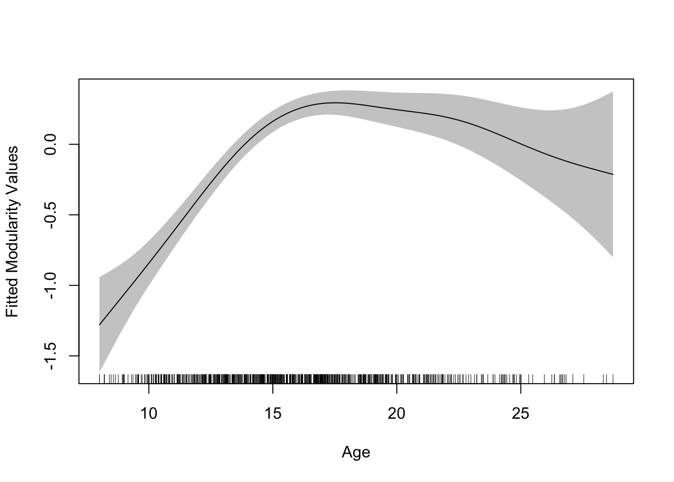
The resulting plot tells a rather interesting story about the developmental trajectory of modularity, with initial increases across early adolescence, a plateauing in mid-adolescence, and then slow declines into young adulthood. However, we can see there is a lot more uncertainty at the later ages (indicated by the sparsity in the hashes in the rug plot).
Latent Curve Model
We will now turn to the longitudinal modeling within the SEM framework, beginning with the latent curve model (or latent growth model; quantitative people aren”t the best with consistent terminology sometimes). Unlike with the mixed-effects models, we will focus on a single package, lavaan, which has become the workhorse of structural equation modeling natively in R (for running SEMs in Mplus using R commands, see the MplusAutomation package). Like with the MLM, we will fit a simple linear growth model using wave as our metric of time. However, unlike with the MLM, time will not appear as a specific variable in the model; rather we code time measurements directly into the factor loadings.
LCM Syntax and Model Fitting
First we will define a model syntax object that specifies the model. While we will cover the basics here, consult the lavaan website for a more complete syntax tutorial.
linear.lcm <- "
              # Define the Latent Variables
              int =~ 1*dlpfc1 + 1*dlpfc2 + 1*dlpfc3 + 1*dlpfc4
              slp =~ 0*dlpfc1 + 1*dlpfc2 + 2*dlpfc3 + 3*dlpfc4

              # Define Factor Means
              int ~ 1
              slp ~ 1

              # Define Factor (Co)Variances
              int ~~ int
              int ~~ slp
              slp ~~ slp

              # Define Indicator Residual Variances
              dlpfc1 ~~ dlpfc1
              dlpfc2 ~~ dlpfc2
              dlpfc3 ~~ dlpfc3
              dlpfc4 ~~ dlpfc4
"
In the first section, we use the =~ operator to define the latent variables (int is the intercept and slp is the linear slope factor). The intercept factor loadings are set by pre-multiplying the individual indicators (dlpfc1-dlpfc4) by values of \(1\). We define the slope by pre-multiplying the indicators by linearly increasing values. Here we set the first factor loading to \(0\) and each subsequent loading by increasing integers. This has the effect of estimating intercept values that reflect levels of DLPFC activation at the initial observation (where time is coded \(0\)) and a slope effect that is expressed in per-wave units (here this relates to per-year changes). Because of defaults built into the lavaan function growth(), we could estimate the full linear LCM with just these first two lines of code (the Mplus syntax is similarly simple). However, for completeness, we will write out the remainder of the model parameters for this initial model.
The next two sections define the parameters of the latent variables. Here we estimate intercepts (i.e., the fixed or average intercept and slope) using the regression operator (~) with \(1\) on the right hand side and (co)variances using the ~~ operator. Note that variances int ~~ int are just the covariance of a variable with itself (take a shot if that makes your head hurt a little bit). Finally, we can define the residual variances of the indicators using the same ~~ operator.
We can then use the growth() function mentioned previously to fit the syntax we wrote to the executive.function data. Here we will estimate the model with Maximum Likelihood (estimator = "ML") and we will allow for missing data using the missing = "FIML" argument. Standard alternatives might include estimator = "MLR" for Robust Maximum Likelihood if we have non-normal continuous data, or estimator = WLSMV if we have discrete data (see the lavaan webpage for a full list of available options). In general, we will always allow for missing data, but we could change to missing = "listwise" if we wanted to do only complete-case analysis. This option is actually the lavaan default, so users should be cautious that this is intended and review the number of observations used in the model to confirm intended behavior.
lcm <- lavaan::growth(linear.lcm,
                      data = executive.function,
                      estimator = "ML",
                      missing = "FIML")
LCM Outputs
We can then summarize the model output using summary() with some optional arguments. While we will mostly output all of the available information, including fit.measures, raw (estimates) and standardized (standardize) parameter estimates, and rsquare, there might be cases where we are only interested in some subsection of the output. For instance, if we are building a sequence of models, we might only consult fit measures without viewing the parameters and associated inference tests so that our model selection isn”t driven by “peeking” at effects of interest.
summary(lcm, fit.measures = TRUE, estimates = TRUE,
        standardize = TRUE, rsquare = TRUE)
## lavaan 0.6.13 ended normally after 22 iterations
##
## Estimator ML
## Optimization method NLMINB
## Number of model parameters 9
##
## Number of observations 342
## Number of missing patterns 8
##
## Model Test User Model:
##
## Test statistic 1.229
## Degrees of freedom 5
## P-value (Chi-square) 0.942
##
## Model Test Baseline Model:
##
## Test statistic 381.370
## Degrees of freedom 6
## P-value 0.000
##
## User Model versus Baseline Model:
##
## Comparative Fit Index (CFI) 1.000
## Tucker-Lewis Index (TLI) 1.012
##
## Robust Comparative Fit Index (CFI) 1.000
## Robust Tucker-Lewis Index (TLI) 1.012
##
## Loglikelihood and Information Criteria:
##
## Loglikelihood user model (H0) -1735.785
## Loglikelihood unrestricted model (H1) -1735.170
##
## Akaike (AIC) 3489.570
## Bayesian (BIC) 3524.083
## Sample-size adjusted Bayesian (SABIC) 3495.533
##
## Root Mean Square Error of Approximation:
##
## RMSEA 0.000
## 90 Percent confidence interval - lower 0.000
## 90 Percent confidence interval - upper 0.014
## P-value H_0: RMSEA <= 0.050 0.990
## P-value H_0: RMSEA >= 0.080 0.001
##
## Robust RMSEA 0.000
## 90 Percent confidence interval - lower 0.000
## 90 Percent confidence interval - upper 0.018
## P-value H_0: Robust RMSEA <= 0.050 0.988
## P-value H_0: Robust RMSEA >= 0.080 0.001
##
## Standardized Root Mean Square Residual:
##
## SRMR 0.016
##
## Parameter Estimates:
##
## Standard errors Standard
## Information Observed
## Observed information based on Hessian
##
## Latent Variables:
## Estimate Std.Err z-value P(>|z|) Std.lv Std.all
## int =~
## dlpfc1 1.000 0.880 0.878
## dlpfc2 1.000 0.880 0.813
## dlpfc3 1.000 0.880 0.810
## dlpfc4 1.000 0.880 0.820
## slp =~
## dlpfc1 0.000 0.000 0.000
## dlpfc2 1.000 0.287 0.265
## dlpfc3 2.000 0.574 0.528
## dlpfc4 3.000 0.861 0.802
##
## Covariances:
## Estimate Std.Err z-value P(>|z|) Std.lv Std.all
## int ~~
## slp -0.126 0.031 -4.102 0.000 -0.499 -0.499
##
## Intercepts:
## Estimate Std.Err z-value P(>|z|) Std.lv Std.all
## int 0.543 0.053 10.181 0.000 0.617 0.617
## slp 0.121 0.021 5.705 0.000 0.420 0.420
## .dlpfc1 0.000 0.000 0.000
## .dlpfc2 0.000 0.000 0.000
## .dlpfc3 0.000 0.000 0.000
## .dlpfc4 0.000 0.000 0.000
##
## Variances:
## Estimate Std.Err z-value P(>|z|) Std.lv Std.all
## int 0.775 0.086 9.009 0.000 1.000 1.000
## slp 0.082 0.016 5.180 0.000 1.000 1.000
## .dlpfc1 0.231 0.063 3.675 0.000 0.231 0.229
## .dlpfc2 0.568 0.055 10.261 0.000 0.568 0.484
## .dlpfc3 0.582 0.058 10.117 0.000 0.582 0.493
## .dlpfc4 0.393 0.074 5.308 0.000 0.393 0.341
##
## R-Square:
## Estimate
## dlpfc1 0.771
## dlpfc2 0.516
## dlpfc3 0.507
## dlpfc4 0.659One nice thing about fitting our model to the raw data instead of standardizing beforehand is that with the standardize = TRUE argument, we get 3 sets of parameter estimates: the raw scale estimates (under Estimates), the estimates when the latent variables are standardized but the indicators remain in the raw scale (under Std.lv), and the fully standardized solution (under Std.all). In the same spirit of maximizing the information from the model, we can actually re-fit the model using estimator = "MLR". Here we will only output the fit.measures to see how the robust estimator changes our model fit information.
lcm <- lavaan::growth(linear.lcm,
                      data = executive.function,
                      estimator = "MLR",
                      missing = "FIML")

summary(lcm, fit.measures = TRUE, estimates = FALSE,
        standardize = FALSE, rsquare = FALSE)
## lavaan 0.6.13 ended normally after 22 iterations
##
## Estimator ML
## Optimization method NLMINB
## Number of model parameters 9
##
## Number of observations 342
## Number of missing patterns 8
##
## Model Test User Model:
## Standard Scaled
## Test Statistic 1.229 1.139
## Degrees of freedom 5 5
## P-value (Chi-square) 0.942 0.951
## Scaling correction factor 1.079
## Yuan-Bentler correction (Mplus variant)
##
## Model Test Baseline Model:
##
## Test statistic 381.370 305.720
## Degrees of freedom 6 6
## P-value 0.000 0.000
## Scaling correction factor 1.247
##
## User Model versus Baseline Model:
##
## Comparative Fit Index (CFI) 1.000 1.000
## Tucker-Lewis Index (TLI) 1.012 1.015
##
## Robust Comparative Fit Index (CFI) 1.000
## Robust Tucker-Lewis Index (TLI) 1.013
##
## Loglikelihood and Information Criteria:
##
## Loglikelihood user model (H0) -1735.785 -1735.785
## Scaling correction factor 1.135
## for the MLR correction
## Loglikelihood unrestricted model (H1) -1735.170 -1735.170
## Scaling correction factor 1.115
## for the MLR correction
##
## Akaike (AIC) 3489.570 3489.570
## Bayesian (BIC) 3524.083 3524.083
## Sample-size adjusted Bayesian (SABIC) 3495.533 3495.533
##
## Root Mean Square Error of Approximation:
##
## RMSEA 0.000 0.000
## 90 Percent confidence interval - lower 0.000 0.000
## 90 Percent confidence interval - upper 0.014 0.000
## P-value H_0: RMSEA <= 0.050 0.990 0.994
## P-value H_0: RMSEA >= 0.080 0.001 0.000
##
## Robust RMSEA 0.000
## 90 Percent confidence interval - lower 0.000
## 90 Percent confidence interval - upper 0.008
## P-value H_0: Robust RMSEA <= 0.050 0.988
## P-value H_0: Robust RMSEA >= 0.080 0.001
##
## Standardized Root Mean Square Residual:
##
## SRMR 0.016 0.016We can see that we get a new column of robust fit statistics to accompany the standard measures which correct for the non-normality in our data. In this case, our data are not too non-normal and so there is little difference. However, this will not always be the case. To vastly over-simplify, we are looking to see if our Model Test User Model: test statistic is non-significant. However, be aware that this test is over-powered and will often be significant in large samples, even in a well fitting model. We also tend to look for CFI/TLI \(> 0.95\), RMSEA \(< 0.05\), and SRMR \(< 0.08\) to indicate an excellent model fit. While these cutoff values are somewhat arbitrary, they can serve as a rough huristic, and the linear LCM more than satisfies each of these criteria. For more discussion of fit indices, consult the resources outlined in the main text. We can now jump back and orient to the parameter estimate output.
summary(lcm, fit.measures = FALSE, estimates=  TRUE,
        standardize = TRUE, rsquare = TRUE)
## lavaan 0.6.13 ended normally after 22 iterations
##
## Estimator ML
## Optimization method NLMINB
## Number of model parameters 9
##
## Number of observations 342
## Number of missing patterns 8
##
## Model Test User Model:
## Standard Scaled
## Test Statistic 1.229 1.139
## Degrees of freedom 5 5
## P-value (Chi-square) 0.942 0.951
## Scaling correction factor 1.079
## Yuan-Bentler correction (Mplus variant)
##
## Parameter Estimates:
##
## Standard errors Sandwich
## Information bread Observed
## Observed information based on Hessian
##
## Latent Variables:
## Estimate Std.Err z-value P(>|z|) Std.lv Std.all
## int =~
## dlpfc1 1.000 0.880 0.878
## dlpfc2 1.000 0.880 0.813
## dlpfc3 1.000 0.880 0.810
## dlpfc4 1.000 0.880 0.820
## slp =~
## dlpfc1 0.000 0.000 0.000
## dlpfc2 1.000 0.287 0.265
## dlpfc3 2.000 0.574 0.528
## dlpfc4 3.000 0.861 0.802
##
## Covariances:
## Estimate Std.Err z-value P(>|z|) Std.lv Std.all
## int ~~
## slp -0.126 0.037 -3.406 0.001 -0.499 -0.499
##
## Intercepts:
## Estimate Std.Err z-value P(>|z|) Std.lv Std.all
## int 0.543 0.053 10.180 0.000 0.617 0.617
## slp 0.121 0.021 5.704 0.000 0.420 0.420
## .dlpfc1 0.000 0.000 0.000
## .dlpfc2 0.000 0.000 0.000
## .dlpfc3 0.000 0.000 0.000
## .dlpfc4 0.000 0.000 0.000
##
## Variances:
## Estimate Std.Err z-value P(>|z|) Std.lv Std.all
## int 0.775 0.093 8.335 0.000 1.000 1.000
## slp 0.082 0.017 4.761 0.000 1.000 1.000
## .dlpfc1 0.231 0.075 3.060 0.002 0.231 0.229
## .dlpfc2 0.568 0.057 9.884 0.000 0.568 0.484
## .dlpfc3 0.582 0.062 9.332 0.000 0.582 0.493
## .dlpfc4 0.393 0.076 5.138 0.000 0.393 0.341
##
## R-Square:
## Estimate
## dlpfc1 0.771
## dlpfc2 0.516
## dlpfc3 0.507
## dlpfc4 0.659The first section of parameters Latent Variables: is of little interest to us for now since we pre-determined these factor loadings as a part of our model (but maybe check that they are the values you expect) and there are therefore no inferential tests on these parameters. The Covariances: section shows us the covariance (and correlation if we asked for standardized results) between the intercept and slope. Here we can see that the correlation is strong and negative (\(r = -0.499\)) suggesting that those with the lowest initial levels of DLPFC activation tend to show the strongest increases in activation over time.
The Intercepts: section shows us the means of the latent factors and would show the conditional (denoted by a . before a variable name) intercepts of the indicators, but we do not estimate these values in a growth model (rather the means are reproduced by the factor means through the loadings, \(\mathbf{\alpha\Lambda}\)). Here we can see that the average activation at the initial timepoint is \(0.543\) and the average rate of change is \(0.121\) units per wave, both of which are significant.
Next we have the factor variances and the indicator residual (again denoted with .) variances in the Variances: section. The variances of the intercept and slope are significant suggesting there are meaningful individual differences in initial level and rate of change over time. The residual variances comprise the variance of the indicator not accounted for by the latent variables in the model.
Finally, we have the R-Square: section where the proportion of variance explained in each of the endogenous variables (here just the indicators but this could contain other endogenous observed or latent variables in other models). Conveniently, this is simply \(1\) minus the standardized residual variance for each item.
We can output these parameters in a slightly more compact format using the tidy() function from the broom package and pass it to the kable() function from the kableExtra package to output a table in the "html" format. If we were writing a manuscript, we might alternatively wish to output the rmarkdown in PDF form and use the format = "latex" argument.
broom::tidy(lcm) %>%
  select(-op, -std.nox) %>%
  kableExtra::kable(label = NA,
                    format = "html",
                    digits = 3,
                    booktabs = TRUE,
                    escape = FALSE,
                    caption = "**Linear Latent Curve Model**",
                    align = "c",
                    col.names=c("Parameter", "Estimate", "SE", "Statistic",
                                "*p*-value", "Std.LV", "Std.All"),
                    row.names = FALSE) %>%
kableExtra::row_spec(row = 0, align = "c")| Parameter | Estimate | SE | Statistic | p-value | Std.LV | Std.All |
|---|---|---|---|---|---|---|
| int =~ dlpfc1 | 1.000 | 0.000 | NA | NA | 0.880 | 0.878 |
| int =~ dlpfc2 | 1.000 | 0.000 | NA | NA | 0.880 | 0.813 |
| int =~ dlpfc3 | 1.000 | 0.000 | NA | NA | 0.880 | 0.810 |
| int =~ dlpfc4 | 1.000 | 0.000 | NA | NA | 0.880 | 0.820 |
| slp =~ dlpfc1 | 0.000 | 0.000 | NA | NA | 0.000 | 0.000 |
| slp =~ dlpfc2 | 1.000 | 0.000 | NA | NA | 0.287 | 0.265 |
| slp =~ dlpfc3 | 2.000 | 0.000 | NA | NA | 0.574 | 0.528 |
| slp =~ dlpfc4 | 3.000 | 0.000 | NA | NA | 0.861 | 0.802 |
| int ~1 | 0.543 | 0.053 | 10.180 | 0.000 | 0.617 | 0.617 |
| slp ~1 | 0.121 | 0.021 | 5.704 | 0.000 | 0.420 | 0.420 |
| int ~~ int | 0.775 | 0.093 | 8.335 | 0.000 | 1.000 | 1.000 |
| int ~~ slp | -0.126 | 0.037 | -3.406 | 0.001 | -0.499 | -0.499 |
| slp ~~ slp | 0.082 | 0.017 | 4.761 | 0.000 | 1.000 | 1.000 |
| dlpfc1 ~~ dlpfc1 | 0.231 | 0.075 | 3.060 | 0.002 | 0.231 | 0.229 |
| dlpfc2 ~~ dlpfc2 | 0.568 | 0.057 | 9.884 | 0.000 | 0.568 | 0.484 |
| dlpfc3 ~~ dlpfc3 | 0.582 | 0.062 | 9.332 | 0.000 | 0.582 | 0.493 |
| dlpfc4 ~~ dlpfc4 | 0.393 | 0.076 | 5.138 | 0.000 | 0.393 | 0.341 |
| dlpfc1 ~1 | 0.000 | 0.000 | NA | NA | 0.000 | 0.000 |
| dlpfc2 ~1 | 0.000 | 0.000 | NA | NA | 0.000 | 0.000 |
| dlpfc3 ~1 | 0.000 | 0.000 | NA | NA | 0.000 | 0.000 |
| dlpfc4 ~1 | 0.000 | 0.000 | NA | NA | 0.000 | 0.000 |
LCM Path Diagrams
We might also wish to generate a diagram visualization of the LCM model, either for model checking or for presenting results. We can use the semPaths() function from the semPlot package to do just that. Here we will plot the model results including the intercepts and with black paths. The what argument we will set to "est" to scale the size of the paths to the parameter estimate.
semPlot::semPaths(lcm,
                  what = "est",
                  intercepts = TRUE,
                  edge.color = "black")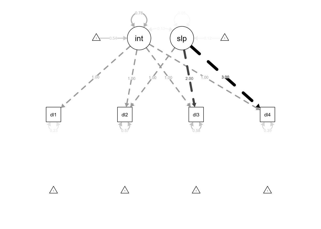
However, we can see that this path scaling is a little unfortunate because the integer factor loadings sort of swamp out the parameters we are primarily interested in. Instead we can change this argument to what = "paths" to have equally-sized paths, and then label those paths with the parameters using whatLabels = "est" (or whatLabels = "std" for standardized estimates).
semPlot::semPaths(lcm,
                  what = "paths",
                  whatLabels = "est",
                  intercepts = TRUE,
                  edge.color = "black")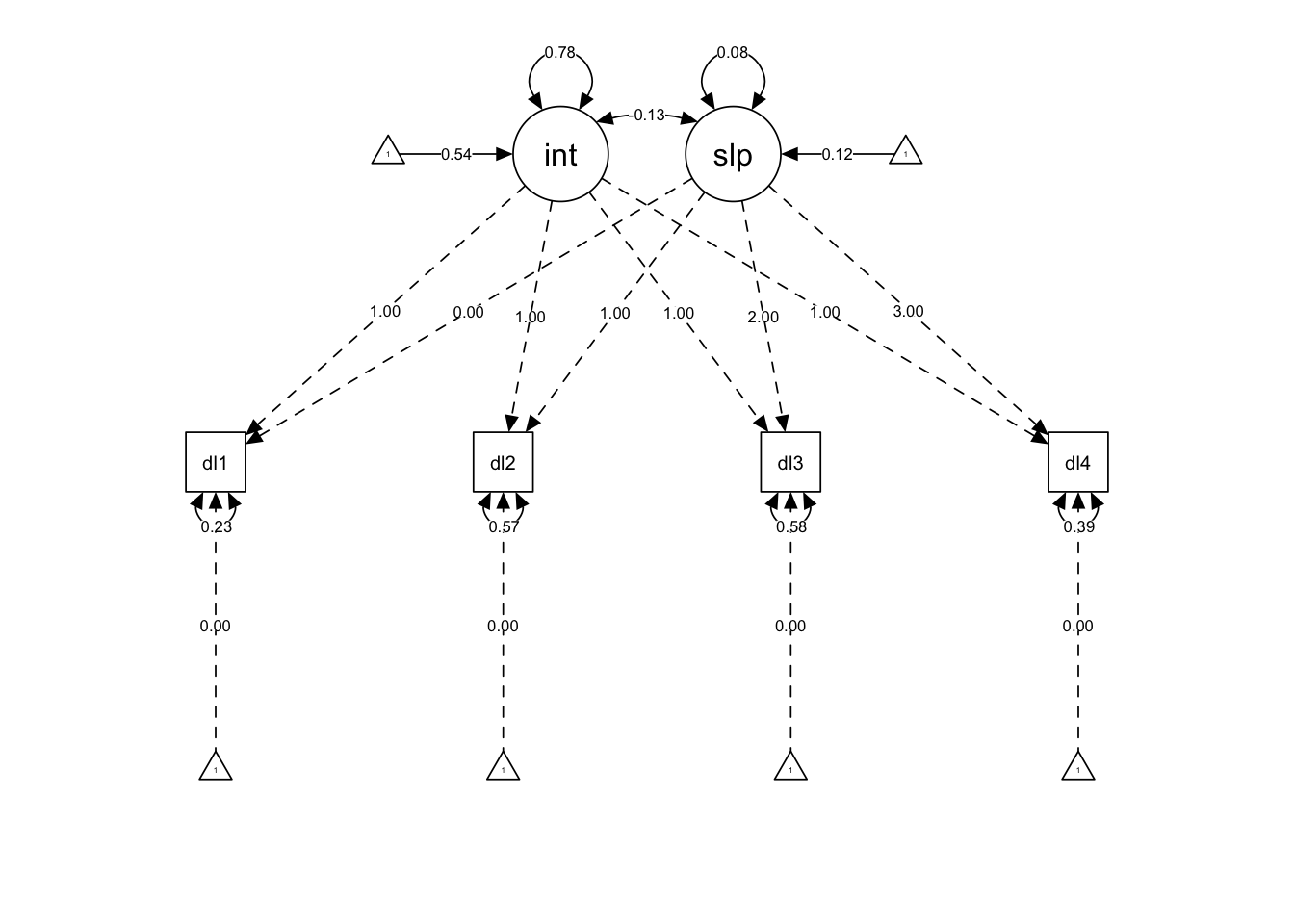
Much better… By standard convention, latent variables are represented as circles, observed variables as squares, regression paths as straight single-headed arrows, and (co)variances as curved double-headed arrows. Parameters that are set to particular values rather than estimated (e.g., factor loadings here and indicator intercepts) are displayed with dashed lines.
LCM Plotting Model-Implied Trajectories
Finally, like with the MLM, we might want to plot model-implied individual trajectories of DLPFC activation. We have to do a little data management song and dance to get the predicted values and then convert to long format (which we do within the ggplot() function directly instead of creating a new dataframe to store in memory), but the results are the same as before.
ggplot2::ggplot(data.frame(id=lcm@Data@case.idx[[1]],
                           lavPredict(lcm,type="ov")) %>%
                  pivot_longer(cols = starts_with("dlpfc"),
                               names_to = c(".value", "wave"),
                               names_pattern = "(.+)(.)") %>%
                  dplyr::mutate(wave = as.numeric(wave)),
                aes(x = wave,
                    y = dlpfc,
                    group = id,
                    color = factor(id))) +
  geom_line() +
  labs(title = "Canonical LCM Trajectories",
       x = "Wave",
       y = "Predicted DLFPC Activation") +
theme(legend.position = "none") 
Latent Change Score Model
Finally, we can turn the LCSM parameterization of the linear growth model. Like the LCM, the time predictor will not appear in our model syntax, but even more strangely (at first), neither will any values of time. Rather we will sum across latent change factors to estimate the slope across time.
Linear LCSM
The main complication of the LCSM syntax relative to what we saw with the LCM is that we need to generate phantom variables from the indicators and then relate them with fixed path coefficients to the latent change factors.
linear.lcsm <- "
               # Define Phantom Variables (p = phantom)
               pdlpfc1 =~ 1*dlpfc1; dlpfc1 ~ 0; dlpfc1 ~~ dlpfc1; pdlpfc1 ~~ 0*pdlpfc1
               pdlpfc2 =~ 1*dlpfc2; dlpfc2 ~ 0; dlpfc2 ~~ dlpfc2; pdlpfc2 ~~ 0*pdlpfc2
               pdlpfc3 =~ 1*dlpfc3; dlpfc3 ~ 0; dlpfc3 ~~ dlpfc3; pdlpfc3 ~~ 0*pdlpfc3
               pdlpfc4 =~ 1*dlpfc4; dlpfc4 ~ 0; dlpfc4 ~~ dlpfc4; pdlpfc4 ~~ 0*pdlpfc4

               # Regressions Between Adjacent Observations
               pdlpfc2 ~ 1*pdlpfc1
               pdlpfc3 ~ 1*pdlpfc2
               pdlpfc4 ~ 1*pdlpfc3

               # Define Change Latent Variables (delta)
               delta21 =~ 1*pdlpfc2; delta21 ~~ 0*delta21
               delta32 =~ 1*pdlpfc3; delta32 ~~ 0*delta32
               delta43 =~ 1*pdlpfc4; delta43 ~~ 0*delta43

               # Define Intercept and Slope
               int =~ 1*pdlpfc1
               slp =~ 1*delta21 + 1*delta32 + 1*delta43

               int ~ 1
               slp ~ 1

               int ~~ slp
               slp ~~ slp
"
In the first section, we define the phantoms (e.g., pdlpfc1) with four commands (separated by ; for compactness): 1) define the phantom by the indicator with a factor loading of \(1\) (pdlpfc1 =~ 1*dlpfc1), 2) set the intercept of the indicator to \(0\) (dlpfc1 ~ 0), 3) estimate the residual variance of the indicator (dlpfc1 ~~ dlpfc1), and set the variance of the phatom to \(0\) (pdlpfc1 ~~ 0*pdlpfc1). This, in effect, pushes the characteristics we need from the indicator variable to the phantom, which facilitates the model.
In the nexttwo sections, we set regressions of \(\gamma = 1\) between adjacent phantoms variables, define the latent change factor by the phantoms after the initial time point (e.g., delta21 =~ 1*pdlpfc2), and set the variance of the latent change factor to zero. This may not be apparent at first blush, but the regressions of \(1\) between adjacent timepoints essentially push the differences in the outcome between observations up into the latent change factors (i.e., what is left over after residualizing out the prior observation).
Finally, we have the final definition of the intercept and slope factors. However, unlike the LCM, the intercept factor is only estimated from the initial phantom variable. The slope factor is defined from the latent change factors, but instead of linear factor loadings, all of these loadings are \(1\) (this sums across the latent changes to give the overall linear trajectory).
Like before, we will take this syntax object and use it to fit the model we specify. Unlike the LCM, we will use the sem() function instead because the growth() defaults won”t serve our purposes with the LCSM. Otherwise, the arguments we will invoke will be the same. While we display it for completeness, we will not spend much time on this output as it exactly recreates the estimates for the LCM we already walked through (we promise; or scroll back up and check). We generate a path diagram for this model as well, but do not display parameter estimates to reduce clutter.
lcsm.linear <- sem(linear.lcsm,
                   data = executive.function,
                   estimator = "ML",
                   missing = "FIML")

summary(lcsm.linear, fit.measures = TRUE, estimates = TRUE, standardize = TRUE, rsquare = TRUE)
## lavaan 0.6.13 ended normally after 22 iterations
##
## Estimator ML
## Optimization method NLMINB
## Number of model parameters 9
##
## Number of observations 342
## Number of missing patterns 8
##
## Model Test User Model:
##
## Test statistic 1.229
## Degrees of freedom 5
## P-value (Chi-square) 0.942
##
## Model Test Baseline Model:
##
## Test statistic 381.370
## Degrees of freedom 6
## P-value 0.000
##
## User Model versus Baseline Model:
##
## Comparative Fit Index (CFI) 1.000
## Tucker-Lewis Index (TLI) 1.012
##
## Robust Comparative Fit Index (CFI) 1.000
## Robust Tucker-Lewis Index (TLI) 1.012
##
## Loglikelihood and Information Criteria:
##
## Loglikelihood user model (H0) -1735.785
## Loglikelihood unrestricted model (H1) -1735.170
##
## Akaike (AIC) 3489.570
## Bayesian (BIC) 3524.083
## Sample-size adjusted Bayesian (SABIC) 3495.533
##
## Root Mean Square Error of Approximation:
##
## RMSEA 0.000
## 90 Percent confidence interval - lower 0.000
## 90 Percent confidence interval - upper 0.014
## P-value H_0: RMSEA <= 0.050 0.990
## P-value H_0: RMSEA >= 0.080 0.001
##
## Robust RMSEA 0.000
## 90 Percent confidence interval - lower 0.000
## 90 Percent confidence interval - upper 0.018
## P-value H_0: Robust RMSEA <= 0.050 0.988
## P-value H_0: Robust RMSEA >= 0.080 0.001
##
## Standardized Root Mean Square Residual:
##
## SRMR 0.016
##
## Parameter Estimates:
##
## Standard errors Standard
## Information Observed
## Observed information based on Hessian
##
## Latent Variables:
## Estimate Std.Err z-value P(>|z|) Std.lv Std.all
## pdlpfc1 =~
## dlpfc1 1.000 0.880 0.878
## pdlpfc2 =~
## dlpfc2 1.000 0.778 0.718
## pdlpfc3 =~
## dlpfc3 1.000 0.775 0.712
## pdlpfc4 =~
## dlpfc4 1.000 0.872 0.812
## delta21 =~
## pdlpfc2 1.000 0.369 0.369
## delta32 =~
## pdlpfc3 1.000 0.370 0.370
## delta43 =~
## pdlpfc4 1.000 0.329 0.329
## int =~
## pdlpfc1 1.000 1.000 1.000
## slp =~
## delta21 1.000 1.000 1.000
## delta32 1.000 1.000 1.000
## delta43 1.000 1.000 1.000
##
## Regressions:
## Estimate Std.Err z-value P(>|z|) Std.lv Std.all
## pdlpfc2 ~
## pdlpfc1 1.000 1.132 1.132
## pdlpfc3 ~
## pdlpfc2 1.000 1.004 1.004
## pdlpfc4 ~
## pdlpfc3 1.000 0.889 0.889
##
## Covariances:
## Estimate Std.Err z-value P(>|z|) Std.lv Std.all
## int ~~
## slp -0.126 0.031 -4.102 0.000 -0.499 -0.499
##
## Intercepts:
## Estimate Std.Err z-value P(>|z|) Std.lv Std.all
## .dlpfc1 0.000 0.000 0.000
## .dlpfc2 0.000 0.000 0.000
## .dlpfc3 0.000 0.000 0.000
## .dlpfc4 0.000 0.000 0.000
## int 0.543 0.053 10.181 0.000 0.617 0.617
## slp 0.121 0.021 5.705 0.000 0.420 0.420
## .pdlpfc1 0.000 0.000 0.000
## .pdlpfc2 0.000 0.000 0.000
## .pdlpfc3 0.000 0.000 0.000
## .pdlpfc4 0.000 0.000 0.000
## .delta21 0.000 0.000 0.000
## .delta32 0.000 0.000 0.000
## .delta43 0.000 0.000 0.000
##
## Variances:
## Estimate Std.Err z-value P(>|z|) Std.lv Std.all
## .dlpfc1 0.231 0.063 3.675 0.000 0.231 0.229
## .pdlpfc1 0.000 0.000 0.000
## .dlpfc2 0.568 0.055 10.261 0.000 0.568 0.484
## .pdlpfc2 0.000 0.000 0.000
## .dlpfc3 0.582 0.058 10.117 0.000 0.582 0.493
## .pdlpfc3 0.000 0.000 0.000
## .dlpfc4 0.393 0.074 5.308 0.000 0.393 0.341
## .pdlpfc4 0.000 0.000 0.000
## .delta21 0.000 0.000 0.000
## .delta32 0.000 0.000 0.000
## .delta43 0.000 0.000 0.000
## slp 0.082 0.016 5.180 0.000 1.000 1.000
## int 0.775 0.086 9.009 0.000 1.000 1.000
##
## R-Square:
## Estimate
## dlpfc1 0.771
## pdlpfc1 1.000
## dlpfc2 0.516
## pdlpfc2 1.000
## dlpfc3 0.507
## pdlpfc3 1.000
## dlpfc4 0.659
## pdlpfc4 1.000
## delta21 1.000
## delta32 1.000
## delta43 1.000broom::tidy(lcsm.linear) %>%
arrange(op) %>%
select(-op, -std.nox) %>%
kableExtra::kable(label = NA,
format = "html",
digits = 3,
booktabs = TRUE,
escape = FALSE,
caption = "**Linear Latent Change Score Model**",
align = "c",
col.names=c("Parameter", "Estimate", "SE", "Statistic",
"*p*-value", "Std.LV", "Std.All"),
row.names = FALSE) %>%
kableExtra::row_spec(row = 0, align = "c")| Parameter | Estimate | SE | Statistic | p-value | Std.LV | Std.All |
|---|---|---|---|---|---|---|
| pdlpfc1 =~ dlpfc1 | 1.000 | 0.000 | NA | NA | 0.880 | 0.878 |
| pdlpfc2 =~ dlpfc2 | 1.000 | 0.000 | NA | NA | 0.778 | 0.718 |
| pdlpfc3 =~ dlpfc3 | 1.000 | 0.000 | NA | NA | 0.775 | 0.712 |
| pdlpfc4 =~ dlpfc4 | 1.000 | 0.000 | NA | NA | 0.872 | 0.812 |
| delta21 =~ pdlpfc2 | 1.000 | 0.000 | NA | NA | 0.369 | 0.369 |
| delta32 =~ pdlpfc3 | 1.000 | 0.000 | NA | NA | 0.370 | 0.370 |
| delta43 =~ pdlpfc4 | 1.000 | 0.000 | NA | NA | 0.329 | 0.329 |
| int =~ pdlpfc1 | 1.000 | 0.000 | NA | NA | 1.000 | 1.000 |
| slp =~ delta21 | 1.000 | 0.000 | NA | NA | 1.000 | 1.000 |
| slp =~ delta32 | 1.000 | 0.000 | NA | NA | 1.000 | 1.000 |
| slp =~ delta43 | 1.000 | 0.000 | NA | NA | 1.000 | 1.000 |
| pdlpfc2 ~ pdlpfc1 | 1.000 | 0.000 | NA | NA | 1.132 | 1.132 |
| pdlpfc3 ~ pdlpfc2 | 1.000 | 0.000 | NA | NA | 1.004 | 1.004 |
| pdlpfc4 ~ pdlpfc3 | 1.000 | 0.000 | NA | NA | 0.889 | 0.889 |
| dlpfc1 ~1 | 0.000 | 0.000 | NA | NA | 0.000 | 0.000 |
| dlpfc2 ~1 | 0.000 | 0.000 | NA | NA | 0.000 | 0.000 |
| dlpfc3 ~1 | 0.000 | 0.000 | NA | NA | 0.000 | 0.000 |
| dlpfc4 ~1 | 0.000 | 0.000 | NA | NA | 0.000 | 0.000 |
| int ~1 | 0.543 | 0.053 | 10.181 | 0 | 0.617 | 0.617 |
| slp ~1 | 0.121 | 0.021 | 5.705 | 0 | 0.420 | 0.420 |
| pdlpfc1 ~1 | 0.000 | 0.000 | NA | NA | 0.000 | 0.000 |
| pdlpfc2 ~1 | 0.000 | 0.000 | NA | NA | 0.000 | 0.000 |
| pdlpfc3 ~1 | 0.000 | 0.000 | NA | NA | 0.000 | 0.000 |
| pdlpfc4 ~1 | 0.000 | 0.000 | NA | NA | 0.000 | 0.000 |
| delta21 ~1 | 0.000 | 0.000 | NA | NA | 0.000 | 0.000 |
| delta32 ~1 | 0.000 | 0.000 | NA | NA | 0.000 | 0.000 |
| delta43 ~1 | 0.000 | 0.000 | NA | NA | 0.000 | 0.000 |
| dlpfc1 ~~ dlpfc1 | 0.231 | 0.063 | 3.675 | 0 | 0.231 | 0.229 |
| pdlpfc1 ~~ pdlpfc1 | 0.000 | 0.000 | NA | NA | 0.000 | 0.000 |
| dlpfc2 ~~ dlpfc2 | 0.568 | 0.055 | 10.261 | 0 | 0.568 | 0.484 |
| pdlpfc2 ~~ pdlpfc2 | 0.000 | 0.000 | NA | NA | 0.000 | 0.000 |
| dlpfc3 ~~ dlpfc3 | 0.582 | 0.058 | 10.117 | 0 | 0.582 | 0.493 |
| pdlpfc3 ~~ pdlpfc3 | 0.000 | 0.000 | NA | NA | 0.000 | 0.000 |
| dlpfc4 ~~ dlpfc4 | 0.393 | 0.074 | 5.308 | 0 | 0.393 | 0.341 |
| pdlpfc4 ~~ pdlpfc4 | 0.000 | 0.000 | NA | NA | 0.000 | 0.000 |
| delta21 ~~ delta21 | 0.000 | 0.000 | NA | NA | 0.000 | 0.000 |
| delta32 ~~ delta32 | 0.000 | 0.000 | NA | NA | 0.000 | 0.000 |
| delta43 ~~ delta43 | 0.000 | 0.000 | NA | NA | 0.000 | 0.000 |
| int ~~ slp | -0.126 | 0.031 | -4.102 | 0 | -0.499 | -0.499 |
| slp ~~ slp | 0.082 | 0.016 | 5.180 | 0 | 1.000 | 1.000 |
| int ~~ int | 0.775 | 0.086 | 9.009 | 0 | 1.000 | 1.000 |
semPlot::semPaths(lcsm.linear,
                  layout = "tree2",
                  intercepts = FALSE,
                  edge.color = "black")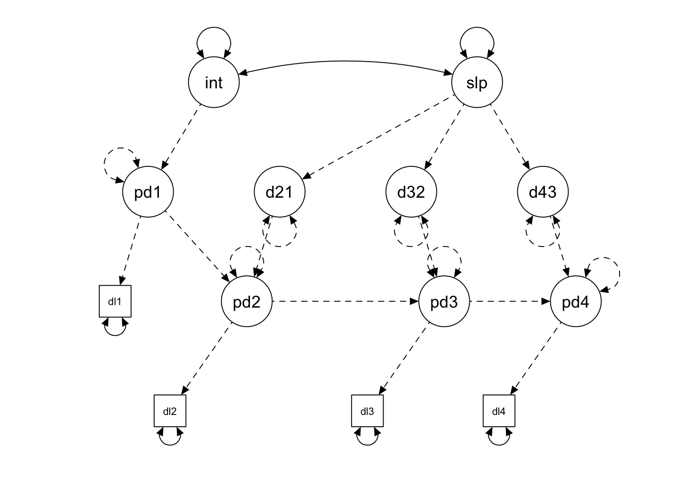
Linear LCSM with Proportional Change
To a first approximation, the model above is an overly complicated method for estimating the same model we could do with two lines in the LCM. However, this parameterization allows us to include effects that are not possible to include in the LCM. To model proportional change, we regression the latent change factor on the prior timepoint phantom variable (delta21 ~ pdlpfc1). This effect tests how change between timepoints depends on prior level on the outcome of interest, and can be used to model interesting non-linearities (especially exponential trends). While not strictly necessary, it is common practice to create an equality constraint across all proportional effects. Here we accomplish this constraint by pre-multiplying all of these regressions with the same label (beta). The rest of the syntax remains the same as above.
proportional.lcsm <- "
               # Define Phantom Variables (p = phantom)
               pdlpfc1 =~ 1*dlpfc1; dlpfc1 ~ 0; dlpfc1 ~~ dlpfc1; pdlpfc1 ~~ 0*pdlpfc1
               pdlpfc2 =~ 1*dlpfc2; dlpfc2 ~ 0; dlpfc2 ~~ dlpfc2; pdlpfc2 ~~ 0*pdlpfc2
               pdlpfc3 =~ 1*dlpfc3; dlpfc3 ~ 0; dlpfc3 ~~ dlpfc3; pdlpfc3 ~~ 0*pdlpfc3
               pdlpfc4 =~ 1*dlpfc4; dlpfc4 ~ 0; dlpfc4 ~~ dlpfc4; pdlpfc4 ~~ 0*pdlpfc4

               # Regressions Between Adjacent Observations
               pdlpfc2 ~ 1*pdlpfc1
               pdlpfc3 ~ 1*pdlpfc2
               pdlpfc4 ~ 1*pdlpfc3

               # Define Change Latent Variables (delta)
               delta21 =~ 1*pdlpfc2; delta21 ~~ 0*delta21
               delta32 =~ 1*pdlpfc3; delta32 ~~ 0*delta32
               delta43 =~ 1*pdlpfc4; delta43 ~~ 0*delta43

               # Define Proportional Change Regressions (beta = equality constraint)
               delta21 ~ beta*pdlpfc1
               delta32 ~ beta*pdlpfc2
               delta43 ~ beta*pdlpfc3

               # Define Intercept and Slope
               int =~ 1*pdlpfc1
               slp =~ 1*delta21 + 1*delta32 + 1*delta43

               int ~ 1
               slp ~ 1

               int ~~ slp
               slp ~~ slp
"

lcsm.proportional <- sem(proportional.lcsm,
                         data = executive.function,
                         estimator = "ML",
                         missing = "FIML")
We will just focus here on the parameter estimate for the proportional effect (beta), which is negative, but non-significant (\(\gamma = -0.090, SE = 0.276, p = 0.745\)). If we were to interpret this parameter, we would say that those with higher levels at prior timepoints tend to show less positive changes between adjacent timepoints (we would need to interpret these in light of the fixed effects to be certain if this is smaller increases or greater decreases). Interestingly, note that this is similar in kind to the factor covariance we interpreted in the LCM. If we examine that same parameter here, we can see that the correlation has been attenuated (\(r = -0.295\)) and is now non-significant. Indeed all the parameter estimates have now changed because we have introduced this new proportional effect.
summary(lcsm.proportional, fit.measures = FALSE, estimates = TRUE,
        standardize = FALSE, rsquare = FALSE)
## lavaan 0.6.13 ended normally after 32 iterations
##
## Estimator ML
## Optimization method NLMINB
## Number of model parameters 12
## Number of equality constraints 2
##
## Number of observations 342
## Number of missing patterns 8
##
## Model Test User Model:
##
## Test statistic 1.132
## Degrees of freedom 4
## P-value (Chi-square) 0.889
##
## Parameter Estimates:
##
## Standard errors Standard
## Information Observed
## Observed information based on Hessian
##
## Latent Variables:
## Estimate Std.Err z-value P(>|z|)
## pdlpfc1 =~
## dlpfc1 1.000
## pdlpfc2 =~
## dlpfc2 1.000
## pdlpfc3 =~
## dlpfc3 1.000
## pdlpfc4 =~
## dlpfc4 1.000
## delta21 =~
## pdlpfc2 1.000
## delta32 =~
## pdlpfc3 1.000
## delta43 =~
## pdlpfc4 1.000
## int =~
## pdlpfc1 1.000
## slp =~
## delta21 1.000
## delta32 1.000
## delta43 1.000
##
## Regressions:
## Estimate Std.Err z-value P(>|z|)
## pdlpfc2 ~
## pdlpfc1 1.000
## pdlpfc3 ~
## pdlpfc2 1.000
## pdlpfc4 ~
## pdlpfc3 1.000
## delta21 ~
## pdlpfc1 (beta) -0.090 0.276 -0.325 0.745
## delta32 ~
## pdlpfc2 (beta) -0.090 0.276 -0.325 0.745
## delta43 ~
## pdlpfc3 (beta) -0.090 0.276 -0.325 0.745
##
## Covariances:
## Estimate Std.Err z-value P(>|z|)
## int ~~
## slp -0.074 0.162 -0.457 0.647
##
## Intercepts:
## Estimate Std.Err z-value P(>|z|)
## .dlpfc1 0.000
## .dlpfc2 0.000
## .dlpfc3 0.000
## .dlpfc4 0.000
## int 0.540 0.054 9.994 0.000
## slp 0.179 0.183 0.981 0.326
## .pdlpfc1 0.000
## .pdlpfc2 0.000
## .pdlpfc3 0.000
## .pdlpfc4 0.000
## .delta21 0.000
## .delta32 0.000
## .delta43 0.000
##
## Variances:
## Estimate Std.Err z-value P(>|z|)
## .dlpfc1 0.208 0.102 2.043 0.041
## .pdlpfc1 0.000
## .dlpfc2 0.573 0.058 9.820 0.000
## .pdlpfc2 0.000
## .dlpfc3 0.577 0.060 9.570 0.000
## .pdlpfc3 0.000
## .dlpfc4 0.413 0.095 4.358 0.000
## .pdlpfc4 0.000
## .delta21 0.000
## .delta32 0.000
## .delta43 0.000
## slp 0.079 0.016 4.970 0.000
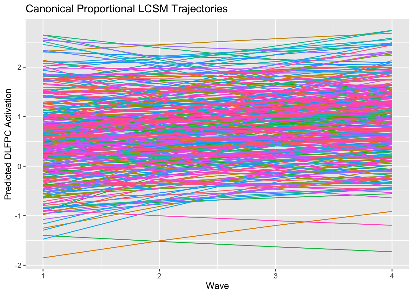
## int 0.796 0.115 6.925 0.000Like before, we can generate tables, a path diagram, and plot model-implied individual trajectories. Note that the proportional model does not generate noticeably non-linear implied trajectories due to the very weak proportional effect.
broom::tidy(lcsm.proportional) %>%
  arrange(op) %>%
  select(-op, -std.nox) %>%
  kableExtra::kable(label = NA,
                    format = "html",
                    digits = 3,
                    booktabs = TRUE,
                    escape = FALSE,
                    caption = "**Linear Latent Change Score Model with Proportional Change**",
                    align = "c",
                    col.names=c("Parameter", "Label", "Estimate", "SE", "Statistic",
                                "*p*-value", "Std.LV", "Std.All"),
                    row.names = FALSE) %>%
kableExtra::row_spec(row = 0, align = "c")| Parameter | Label | Estimate | SE | Statistic | p-value | Std.LV | Std.All |
|---|---|---|---|---|---|---|---|
| pdlpfc1 =~ dlpfc1 | 1.000 | 0.000 | NA | NA | 0.892 | 0.891 | |
| pdlpfc2 =~ dlpfc2 | 1.000 | 0.000 | NA | NA | 0.777 | 0.716 | |
| pdlpfc3 =~ dlpfc3 | 1.000 | 0.000 | NA | NA | 0.776 | 0.714 | |
| pdlpfc4 =~ dlpfc4 | 1.000 | 0.000 | NA | NA | 0.861 | 0.802 | |
| delta21 =~ pdlpfc2 | 1.000 | 0.000 | NA | NA | 0.405 | 0.405 | |
| delta32 =~ pdlpfc3 | 1.000 | 0.000 | NA | NA | 0.370 | 0.370 | |
| delta43 =~ pdlpfc4 | 1.000 | 0.000 | NA | NA | 0.303 | 0.303 | |
| int =~ pdlpfc1 | 1.000 | 0.000 | NA | NA | 1.000 | 1.000 | |
| slp =~ delta21 | 1.000 | 0.000 | NA | NA | 0.895 | 0.895 | |
| slp =~ delta32 | 1.000 | 0.000 | NA | NA | 0.983 | 0.983 | |
| slp =~ delta43 | 1.000 | 0.000 | NA | NA | 1.080 | 1.080 | |
| pdlpfc2 ~ pdlpfc1 | 1.000 | 0.000 | NA | NA | 1.148 | 1.148 | |
| pdlpfc3 ~ pdlpfc2 | 1.000 | 0.000 | NA | NA | 1.002 | 1.002 | |
| pdlpfc4 ~ pdlpfc3 | 1.000 | 0.000 | NA | NA | 0.900 | 0.900 | |
| delta21 ~ pdlpfc1 | beta | -0.090 | 0.276 | -0.325 | 0.745 | -0.254 | -0.254 |
| delta32 ~ pdlpfc2 | beta | -0.090 | 0.276 | -0.325 | 0.745 | -0.243 | -0.243 |
| delta43 ~ pdlpfc3 | beta | -0.090 | 0.276 | -0.325 | 0.745 | -0.267 | -0.267 |
| dlpfc1 ~1 | 0.000 | 0.000 | NA | NA | 0.000 | 0.000 | |
| dlpfc2 ~1 | 0.000 | 0.000 | NA | NA | 0.000 | 0.000 | |
| dlpfc3 ~1 | 0.000 | 0.000 | NA | NA | 0.000 | 0.000 | |
| dlpfc4 ~1 | 0.000 | 0.000 | NA | NA | 0.000 | 0.000 | |
| int ~1 | 0.540 | 0.054 | 9.994 | 0.000 | 0.605 | 0.605 | |
| slp ~1 | 0.179 | 0.183 | 0.981 | 0.326 | 0.637 | 0.637 | |
| pdlpfc1 ~1 | 0.000 | 0.000 | NA | NA | 0.000 | 0.000 | |
| pdlpfc2 ~1 | 0.000 | 0.000 | NA | NA | 0.000 | 0.000 | |
| pdlpfc3 ~1 | 0.000 | 0.000 | NA | NA | 0.000 | 0.000 | |
| pdlpfc4 ~1 | 0.000 | 0.000 | NA | NA | 0.000 | 0.000 | |
| delta21 ~1 | 0.000 | 0.000 | NA | NA | 0.000 | 0.000 | |
| delta32 ~1 | 0.000 | 0.000 | NA | NA | 0.000 | 0.000 | |
| delta43 ~1 | 0.000 | 0.000 | NA | NA | 0.000 | 0.000 | |
| dlpfc1 ~~ dlpfc1 | 0.208 | 0.102 | 2.043 | 0.041 | 0.208 | 0.207 | |
| pdlpfc1 ~~ pdlpfc1 | 0.000 | 0.000 | NA | NA | 0.000 | 0.000 | |
| dlpfc2 ~~ dlpfc2 | 0.573 | 0.058 | 9.820 | 0.000 | 0.573 | 0.487 | |
| pdlpfc2 ~~ pdlpfc2 | 0.000 | 0.000 | NA | NA | 0.000 | 0.000 | |
| dlpfc3 ~~ dlpfc3 | 0.577 | 0.060 | 9.570 | 0.000 | 0.577 | 0.490 | |
| pdlpfc3 ~~ pdlpfc3 | 0.000 | 0.000 | NA | NA | 0.000 | 0.000 | |
| dlpfc4 ~~ dlpfc4 | 0.413 | 0.095 | 4.358 | 0.000 | 0.413 | 0.357 | |
| pdlpfc4 ~~ pdlpfc4 | 0.000 | 0.000 | NA | NA | 0.000 | 0.000 | |
| delta21 ~~ delta21 | 0.000 | 0.000 | NA | NA | 0.000 | 0.000 | |
| delta32 ~~ delta32 | 0.000 | 0.000 | NA | NA | 0.000 | 0.000 | |
| delta43 ~~ delta43 | 0.000 | 0.000 | NA | NA | 0.000 | 0.000 | |
| int ~~ slp | -0.074 | 0.162 | -0.457 | 0.647 | -0.295 | -0.295 | |
| slp ~~ slp | 0.079 | 0.016 | 4.970 | 0.000 | 1.000 | 1.000 | |
| int ~~ int | 0.796 | 0.115 | 6.925 | 0.000 | 1.000 | 1.000 |
semPlot::semPaths(lcsm.proportional,
                  layout = "tree2",
                  intercepts = FALSE,
                  edge.color = "black")
ggplot2::ggplot(data.frame(id=lcsm.proportional@Data@case.idx[[1]],
                           lavPredict(lcsm.proportional,type="ov")) %>%
                  pivot_longer(cols = starts_with("dlpfc"),
                               names_to = c(".value", "wave"),
                               names_pattern = "(.+)(.)") %>%
                  dplyr::mutate(wave = as.numeric(wave)),
                aes(x = wave,
                    y = dlpfc,
                    group = id,
                    color = factor(id))) +
  geom_line() +
  labs(title = "Canonical Proportional LCSM Trajectories",
       x = "Wave",
       y = "Predicted DLFPC Activation") +
  theme(legend.position = "none")