Time Structure
Now that we have covered the basic forms of each of the four modeling frameworks, we can start thinking more deeply about how to include time in our longitudinal models. We will begin by visualizing different kinds of assessment schedules and how our models might change depending on the structure of our observations. We will read in subsets of datasets that appear elsewhere in this primer codebook that follow each of three exemplar assessment types. The single.cohort and accelerated datasets were drawn from the executive.function and feedback.learning datasets we saw in the canonical models chapter. The multiple.cohort dataset has been drawn from the adversity dataset (for details, see the Datasets chapter), which measures white matter development across 8 waves. These data contain fractional anisotropy (FA) measures derived from the forceps minor (fmin), a white matter tract that spans the hemispheres of the medial prefrontal cortex. We will see this dataset again when we consider predictors in the Covariates chapter.
single.cohort <- read.csv("data/single-cohort.csv", header = TRUE)

multiple.cohort <- read.csv("data/multiple-cohort.csv", header = TRUE)

accelerated <- read.csv("data/accelerated.csv", header = TRUE)
Assessment Schedules
Single Cohort Data
As we cover in the main text, single cohort studies are by far the most common in longitudinal modeling. Below we can plot the assessment schedule for the canonical models we worked with in the last chapter. To declutter the plot, we have selected 50 individuals from the larger dataset and ordered them by their age at the first assessment.
set.seed(12345)
ggplot(single.cohort %>%
         pivot_longer(cols=starts_with("age"),
                      names_to = c(".value", "wave"),
                      names_pattern = "(.+)(.)"),
       aes(x = age, y = id)) +
  geom_line(aes(group = id), size = .5) +
  geom_point(aes(color = as.factor(wave))) +
  labs(x = "Age", y = "Individual", color = "Wave") +
  theme(legend.position = "top")
We can see that there is some noise in the assessment schedule, as individuals are not observed at exactly intervals, however, we can see clear separation in ages between each wave. Because we cover this data extensively in the Canonical Models chapter, we will not show model fits here. However, we should note that because of the structure of this data, age and wave of assessment are highly collinear (and are more so the better job we do at observing individuals at regular intervals). This will impact our considerations about time later.
Multiple Cohort Data
A slightly more complex assessment schedule design is the multiple cohort design. In these designs, we have multiple, discrete ages at the first assessment which vary across cohorts. Here we can plot our multiple.cohort data, which is organized into three cohorts, beginning at ages \(4\), \(5\), and \(6\). While at later ages the cohorts mix somewhat in terms of ages sampled, no individual is observed at consecutive ages. This highlights a key advantage of the multiple cohort design; they can often provide coverage of a wider developmental window without requiring additional subjects or waves of assessment using principles of planned missingness.
ggplot(multiple.cohort %>%
         pivot_longer(cols=starts_with("fmin"),
                      names_to = c(".value", "age"),
                      names_pattern = "(....)(.+)") %>%
         drop_na(fmin) %>%
         mutate(age = as.numeric(age)),
       aes(x = age, y = id)) +
  geom_line(aes(group = id), size = .5) +
  geom_point(aes(color = as.factor(age), shape = factor(cohort)), size=2) +
  labs(x = "Age", y = "Individual", color = "Wave", shape = "Cohort") +
  theme(legend.position = "top") + guides(color = "none")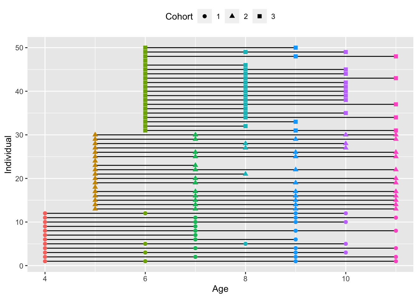
Here we will demonstrate how one might model this type of data using the linear latent curve model for simplicity; however, we could implement this model in any of the 4 modeling frameworks we discussed. To preface the model results, the values of the fmin outcome were normalized to the first age assessed (fmin4) because of the relatively small natural scale of FA values. We have also read in the full adversity data file due to convergence issues with the subsample in multiple.cohort.
mc.wm.model <- "int =~ 1*fmin4 + 1*fmin5 + 1*fmin6 + 1*fmin7 +
                       1*fmin8 + 1*fmin9 + 1*fmin10 + 1*fmin11
                slp =~ 0*fmin4 + 1*fmin5 + 2*fmin6 + 3*fmin7 +
                       4*fmin8 + 5*fmin9 + 6*fmin10 + 7*fmin11
"

mc.wm <- growth(mc.wm.model,
                data = adversity,
                estimator = "ML",
                missing = "FIML")
The real leverage that FIML gives us is apparent using this model. We can measure across \(8\) ages despite no individual having more than \(4\) observations. We can see the abbreviated results below.
summary(mc.wm, fit.measures = FALSE, estimates = TRUE,
        standardize = TRUE, rsquare = FALSE)
## lavaan 0.6.13 ended normally after 33 iterations
##
## Estimator ML
## Optimization method NLMINB
## Number of model parameters 13
##
## Number of observations 398
## Number of missing patterns 40
##
## Model Test User Model:
##
## Test statistic 42.960
## Degrees of freedom 31
## P-value (Chi-square) 0.075
##
## Parameter Estimates:
##
## Standard errors Standard
## Information Observed
## Observed information based on Hessian
##
## Latent Variables:
## Estimate Std.Err z-value P(>|z|) Std.lv Std.all
## int =~
## fmin4 1.000 0.656 0.638
## fmin5 1.000 0.656 0.685
## fmin6 1.000 0.656 0.623
## fmin7 1.000 0.656 0.582
## fmin8 1.000 0.656 0.531
## fmin9 1.000 0.656 0.535
## fmin10 1.000 0.656 0.542
## fmin11 1.000 0.656 0.480
## slp =~
## fmin4 0.000 0.000 0.000
## fmin5 1.000 0.125 0.130
## fmin6 2.000 0.249 0.237
## fmin7 3.000 0.374 0.331
## fmin8 4.000 0.499 0.404
## fmin9 5.000 0.623 0.508
## fmin10 6.000 0.748 0.618
## fmin11 7.000 0.872 0.638
##
## Covariances:
## Estimate Std.Err z-value P(>|z|) Std.lv Std.all
## int ~~
## slp 0.006 0.023 0.276 0.783 0.077 0.077
##
## Intercepts:
## Estimate Std.Err z-value P(>|z|) Std.lv Std.all
## .fmin4 0.000 0.000 0.000
## .fmin5 0.000 0.000 0.000
## .fmin6 0.000 0.000 0.000
## .fmin7 0.000 0.000 0.000
## .fmin8 0.000 0.000 0.000
## .fmin9 0.000 0.000 0.000
## .fmin10 0.000 0.000 0.000
## .fmin11 0.000 0.000 0.000
## int 0.026 0.053 0.485 0.628 0.039 0.039
## slp 0.049 0.012 4.020 0.000 0.393 0.393
##
## Variances:
## Estimate Std.Err z-value P(>|z|) Std.lv Std.all
## .fmin4 0.627 0.141 4.440 0.000 0.627 0.593
## .fmin5 0.458 0.102 4.475 0.000 0.458 0.500
## .fmin6 0.591 0.105 5.646 0.000 0.591 0.533
## .fmin7 0.664 0.091 7.315 0.000 0.664 0.522
## .fmin8 0.796 0.125 6.389 0.000 0.796 0.522
## .fmin9 0.621 0.095 6.565 0.000 0.621 0.413
## .fmin10 0.398 0.116 3.438 0.001 0.398 0.272
## .fmin11 0.589 0.125 4.694 0.000 0.589 0.315
## int 0.431 0.117 3.690 0.000 1.000 1.000
## slp 0.016 0.006 2.685 0.007 1.000 1.000With this model, we will be warned that coverage for certain pairwise combinations is \(< 10\%\), which just reflects the fact that almost no individuals gave data at adjacent ages. We could inspect the model coverage using the lavInspect() function using the argument what = "coverage". Note the values at or near \(0\) on the 1-off diagonal (e.g., fmin5 and fmin4).
lavInspect(mc.wm, what = "coverage")## fmin4 fmin5 fmin6 fmin7 fmin8 fmin9 fmin10 fmin11
## fmin4 0.299
## fmin5 0.000 0.420
## fmin6 0.078 0.000 0.359
## fmin7 0.209 0.264 0.000 0.472
## fmin8 0.030 0.123 0.239 0.008 0.372
## fmin9 0.196 0.204 0.070 0.342 0.003 0.430
## fmin10 0.070 0.113 0.198 0.040 0.244 0.035 0.334
## fmin11 0.151 0.239 0.055 0.342 0.040 0.359 0.030 0.430Finally, we can generate a path diagram, highlighting that the intercept and slope are estimated from all ages even though no individual is measured across all of those ages.
semPaths(mc.wm,
         intercepts = TRUE,
         edge.color = "black")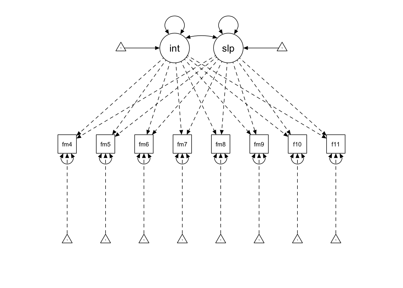
Accelerated Design
The most complex assessment schedule is the accelerated longitudinal design, where no two individual are assessed at the same maturational state (usually age). While it isn’t strictly necessary that we have some smooth continuum of starting ages, accelerated longitudinal studies most often follow this approach. We can see an example below.
set.seed(12345)

ggplot(accelerated %>% group_by(id) %>% filter(length(unique(wave)) == 3) %>%
         ungroup() %>% filter(id %in% sample(id, 100)),
       aes(x = age, y = id)) +
  geom_line(aes(group = id), size = .5) +
  geom_point(aes(color = as.factor(wave))) +
  labs(x = "Age", y = "Individual", color = "Wave", shape = "Cohort") +
  theme(legend.position = "top")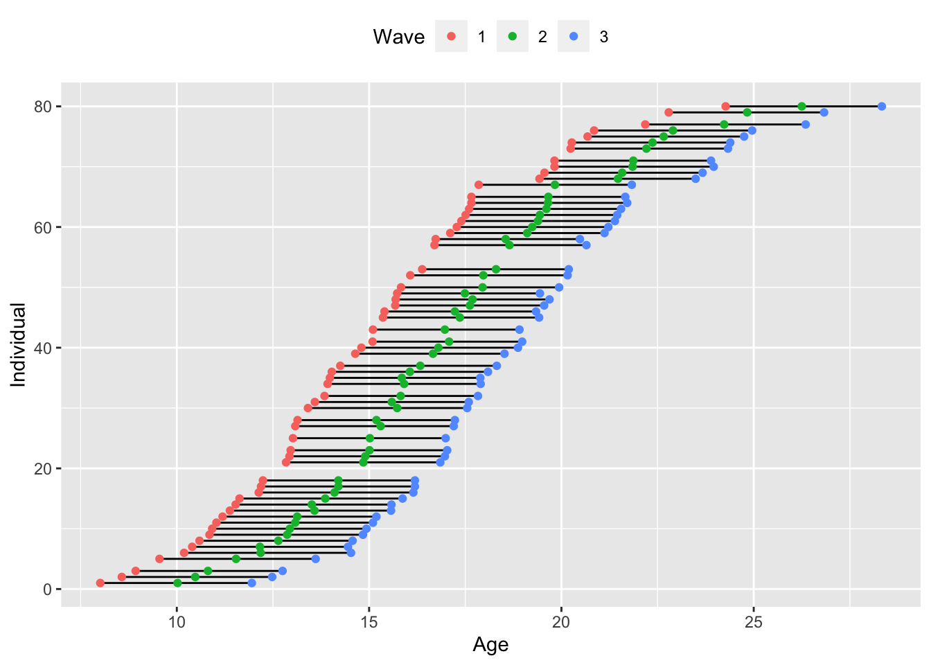
Unlike the single or multiple-cohort data, where we have discrete timepoints of observations, here we have as many as three unique timepoints per person since individuals are unlikely to be the exact same age. While it is possible to fit this type of model using definition variables in an SEM (see the Mplus code for the TSCORE option), it is far more common to fit these assessment schedules with mixed effects models, where we can include precise age into the model as a continuous predictor. We can use the multilevel model to fit a quadratic growth curve to this data. Note that the linear and quadratic effects are fixed effects that are pooled across individuals, and that only the random intercept is included. We could include additional random effects if the data support them, although we would need sufficient numbers of observations within-person to do so.
accel <- lmer(scale(modularity) ~ 1 + age + I(age^2) + (1 | id),
              na.action = na.omit,
              REML = TRUE,
              data = accelerated)
We can see the results of this model below.
summary(accel)## Linear mixed model fit by REML. t-tests use Satterthwaite's method [
## lmerModLmerTest]
## Formula: scale(modularity) ~ 1 + age + I(age^2) + (1 | id)
## Data: accelerated
##
## REML criterion at convergence: 642.4
##
## Scaled residuals:
## Min 1Q Median 3Q Max
## -3.02380 -0.55867 -0.00133 0.56810 2.43080
##
## Random effects:
## Groups Name Variance Std.Dev.
## id (Intercept) 0.4079 0.6386
## Residual 0.5131 0.7163
## Number of obs: 243, groups: id, 81
##
## Fixed effects:
## Estimate Std. Error df t value Pr(>|t|)
## (Intercept) -4.229027 0.928266 239.194448 -4.556 8.32e-06 ***
## age 0.460537 0.105741 239.506334 4.355 1.97e-05 ***
## I(age^2) -0.011828 0.002949 238.656609 -4.011 8.10e-05 ***
## ---
## Signif. codes: 0 '***' 0.001 '**' 0.01 '*' 0.05 '.' 0.1 ' ' 1
##
## Correlation of Fixed Effects:
## (Intr) age
## age -0.982
## I(age^2) 0.940 -0.986If we want to get the overall fixed effects trend, rather than individual trajectories (as we did in the Canonical models), we can use the ggpredict() function from the ggeffects package to generate predicted values of the outcome at specific values of the predictor. This package is especially useful for generating ggplot-compatible dataframes when plotting interactions, but we can still use it for main effects (although a polynomial is a special form of an interaction). We can specify the levels of the predictor within the brackets ([]) or set them to all as we will here to get the full range of ages in our plot. We can then pass this dataframe to ggplot and plot the effect of age with confidence bands shaded.
accel.effects = ggeffects::ggpredict(accel, terms='age [all]')

ggplot(data=accel.effects, aes(x=x,y=predicted)) +
  geom_line() +
  geom_ribbon(aes(ymin=conf.low, ymax=conf.high), alpha=.2) +
  labs(x='Age', y = 'Predicted Learning Rate')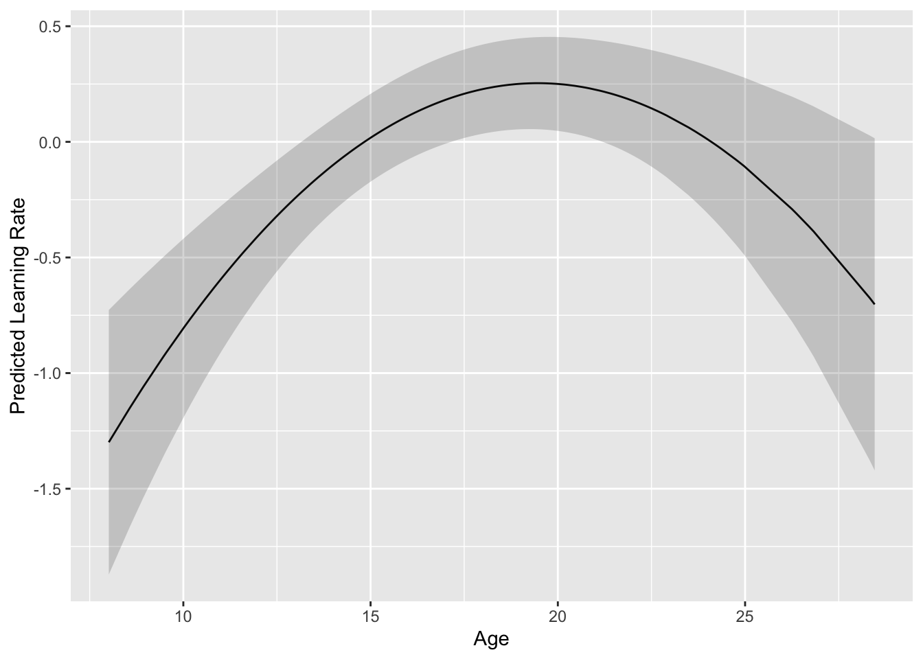
We can see quite a pronounced inverted-U quadratic effect here, with a peak around twenty. While we have this plot here, we might wish to know if the simple linear slope is significant at various points along the curve (i.e., is modularity significantly increasing or decreasing at a given age). To do so, we can use the simple_slopes() function from the interactions package. One quirk is that this function does not recognize a polynomial term like the one we have here. Instead, the function looks for separate variable labels. Well fortunately we can just trick it into working as we would like by duplicating the age variable under a new name (age_temp). We can then re-estimate our model with the interaction of age and our temporary age variable included (i.e., age:age_temp).
accelerated <- accelerated %>% mutate(age_temp = age)

probe.accel <- lmer(scale(modularity) ~ 1 + age + age:age_temp + (1 | id),
                    na.action = na.omit,
                    REML = TRUE,
                    data = accelerated)
We can then pass the new model object to the simple_slopes() function with age as our focal predictor and age_temp as the moderator (of course in this case, it doesn’t matter which variable we put in which position). We can toggle the jnplot argument to TRUE in order to generate a plot of the linear effect of age as a function of age. This plot will show us where within the quadratic curve, we have significant increases or decreases, and where the linear effect is not significant.
interactions::sim_slopes(probe.accel,
                         data = accelerated,
                         pred = age,
                         modx = age_temp,
                         jnplot = TRUE,
                         jnalpha = 0.05)
## JOHNSON-NEYMAN INTERVAL
##
## When age_temp is OUTSIDE the interval [18.79, 27.02], the slope of age is p
## < .05.
##
## Note: The range of observed values of age_temp is [8.01, 28.46]
## SIMPLE SLOPES ANALYSIS
##
## Slope of age when age_temp = 13.14157 (- 1 SD):
##
##   Est.   S.E.   t val.      p
## ------ ------ -------- ------
##   0.10   0.02     4.40   0.00
##
## Slope of age when age_temp = 17.17288 (Mean):
##
##   Est.   S.E.   t val.      p
## ------ ------ -------- ------
##   0.05   0.02     3.01   0.00
##
## Slope of age when age_temp = 21.20419 (+ 1 SD):
##
##   Est.   S.E.   t val.      p
## ------ ------ -------- ------
##   0.01   0.02     0.33   0.74
We can see that from around 19 to 27, the linear effect of age (i.e., the slope of the tangent line) is not significant but is significantly positive before and significantly negative after this age range. We round these numbers because we cannot really think we have such precise measurements to say that linear increases in modularity become non-significant exactly at 18.79. However, this sort of plot can help us distinguish between truly quadratic effects (within increases and decreases) versus a plateauing of the outcome at later ages.
Time Coding
One point of frequent confusion when modeling data (nevermind longitudinal models) is the role of centering the predictors for model results/fit/etc. In general, centering predictors does not change the fundamental information contained within the model, although sometimes it is necessary for practical reason (e.g., reducing collinearity between main effects and product terms). In longitudinal models, the main centering concern is where to place the intercept (i.e., where time is coded 0). While many of our parameter estimates will indeed change based on where we choose to estimate the intercept (most notably the…wait for it…intercept, as well as covariances with the intercept). Here we will demonstrate with the LCM framework since the factor-loading matrix makes what is happening very explicit, but you could replicate these results with any of the other approaches.
First, we can fit the linear model to the single-cohort data we showed above. Here we will place the \(0\) factor loading at the first time point which will result in the intercept reflecting individual differences in the level of the outcome at the initial assessment (i.e., initial status).
initial.status <- "int =~ 1*dlpfc1 + 1*dlpfc2 + 1*dlpfc3 + 1*dlpfc4
                   slp =~ 0*dlpfc1 + 1*dlpfc2 + 2*dlpfc3 + 3*dlpfc4"

initial.status.fit <- growth(initial.status,
                             data = single.cohort,
                             estimator = "ML",
                             missing="FIML")

summary(initial.status.fit, fit.measures = TRUE, estimates = FALSE,
        standardize = FALSE, rsquare = FALSE)
## lavaan 0.6.13 ended normally after 22 iterations
##
## Estimator ML
## Optimization method NLMINB
## Number of model parameters 9
##
## Number of observations 50
## Number of missing patterns 5
##
## Model Test User Model:
##
## Test statistic 12.140
## Degrees of freedom 5
## P-value (Chi-square) 0.033
##
## Model Test Baseline Model:
##
## Test statistic 72.730
## Degrees of freedom 6
## P-value 0.000
##
## User Model versus Baseline Model:
##
## Comparative Fit Index (CFI) 0.893
## Tucker-Lewis Index (TLI) 0.872
##
## Robust Comparative Fit Index (CFI) 0.905
## Robust Tucker-Lewis Index (TLI) 0.886
##
## Loglikelihood and Information Criteria:
##
## Loglikelihood user model (H0) -248.174
## Loglikelihood unrestricted model (H1) -242.104
##
## Akaike (AIC) 514.347
## Bayesian (BIC) 531.555
## Sample-size adjusted Bayesian (SABIC) 503.306
##
## Root Mean Square Error of Approximation:
##
## RMSEA 0.169
## 90 Percent confidence interval - lower 0.045
## 90 Percent confidence interval - upper 0.293
## P-value H_0: RMSEA <= 0.050 0.055
## P-value H_0: RMSEA >= 0.080 0.903
##
## Robust RMSEA 0.173
## 90 Percent confidence interval - lower 0.034
## 90 Percent confidence interval - upper 0.305
## P-value H_0: Robust RMSEA <= 0.050 0.062
## P-value H_0: Robust RMSEA >= 0.080 0.897
##
## Standardized Root Mean Square Residual:
##
## SRMR 0.113We will focus first on fit and then circle back to parameter estimates later. Here the chi-square test statistics is \(12.14\) on \(5%\) degrees of freedom (\(p = 0.033\)), the \(CFI = 0.893\) and the \(RMSEA = 0.169\). We can then re-estimate the model where we code the last factor loading as \(0\) instead so the intercept will represent final status.
final.status <- "int =~ 1*dlpfc1 + 1*dlpfc2 + 1*dlpfc3 + 1*dlpfc4
                 slp =~ -3*dlpfc1 + -2*dlpfc2 + -1*dlpfc3 + 0*dlpfc4"

final.status.fit <- growth(final.status,
                           data = single.cohort,
                           estimator = "ML",
                           missing = "FIML")

summary(final.status.fit, fit.measures = TRUE, estimates = FALSE,
        standardize = FALSE, rsquare = FALSE)
## lavaan 0.6.13 ended normally after 25 iterations
##
## Estimator ML
## Optimization method NLMINB
## Number of model parameters 9
##
## Number of observations 50
## Number of missing patterns 5
##
## Model Test User Model:
##
## Test statistic 12.140
## Degrees of freedom 5
## P-value (Chi-square) 0.033
##
## Model Test Baseline Model:
##
## Test statistic 72.730
## Degrees of freedom 6
## P-value 0.000
##
## User Model versus Baseline Model:
##
## Comparative Fit Index (CFI) 0.893
## Tucker-Lewis Index (TLI) 0.872
##
## Robust Comparative Fit Index (CFI) 0.905
## Robust Tucker-Lewis Index (TLI) 0.886
##
## Loglikelihood and Information Criteria:
##
## Loglikelihood user model (H0) -248.174
## Loglikelihood unrestricted model (H1) -242.104
##
## Akaike (AIC) 514.347
## Bayesian (BIC) 531.555
## Sample-size adjusted Bayesian (SABIC) 503.306
##
## Root Mean Square Error of Approximation:
##
## RMSEA 0.169
## 90 Percent confidence interval - lower 0.045
## 90 Percent confidence interval - upper 0.293
## P-value H_0: RMSEA <= 0.050 0.055
## P-value H_0: RMSEA >= 0.080 0.903
##
## Robust RMSEA 0.173
## 90 Percent confidence interval - lower 0.034
## 90 Percent confidence interval - upper 0.305
## P-value H_0: Robust RMSEA <= 0.050 0.062
## P-value H_0: Robust RMSEA >= 0.080 0.897
##
## Standardized Root Mean Square Residual:
##
## SRMR 0.113Looking at the model fit values, they are exactly identical to the initial status model. We have effectively re-arranged deck chairs on the Titanic (and Rose is about to shove Jack off that door; don’t @ me) as far as model fit goes. So why might we wish to reformulate this model? Well, individual differences in level might be interesting to interpret substantively at one point over another depending on our application of interest. While many research hypotheses will lend themselves naturally to the initial status approach, in intervention work or a training study we might be far more interesting in interpreting where individuals end up (spoken with all the authority of someone who does not do intervention work).
| Parameter | Estimate | SE | Statistic | p-value | Std.LV | Std.All |
|---|---|---|---|---|---|---|
| dlpfc1 ~~ dlpfc1 | 0.280 | 0.196 | 1.427 | 0.154 | 0.280 | 0.307 |
| dlpfc2 ~~ dlpfc2 | 0.459 | 0.140 | 3.275 | 0.001 | 0.459 | 0.435 |
| dlpfc3 ~~ dlpfc3 | 0.389 | 0.128 | 3.039 | 0.002 | 0.389 | 0.368 |
| dlpfc4 ~~ dlpfc4 | 0.640 | 0.278 | 2.302 | 0.021 | 0.640 | 0.428 |
| int ~~ int | 0.631 | 0.207 | 3.039 | 0.002 | 1.000 | 1.000 |
| slp ~~ slp | 0.055 | 0.054 | 1.010 | 0.313 | 1.000 | 1.000 |
| int ~~ slp | -0.045 | 0.097 | -0.467 | 0.641 | -0.243 | -0.243 |
| int ~1 | 0.628 | 0.132 | 4.761 | 0.000 | 0.791 | 0.791 |
| slp ~1 | 0.114 | 0.054 | 2.120 | 0.034 | 0.487 | 0.487 |
| Parameter | Estimate | SE | Statistic | p-value | Std.LV | Std.All |
|---|---|---|---|---|---|---|
| dlpfc1 ~~ dlpfc1 | 0.280 | 0.196 | 1.427 | 0.154 | 0.280 | 0.307 |
| dlpfc2 ~~ dlpfc2 | 0.459 | 0.140 | 3.275 | 0.001 | 0.459 | 0.435 |
| dlpfc3 ~~ dlpfc3 | 0.389 | 0.128 | 3.039 | 0.002 | 0.389 | 0.368 |
| dlpfc4 ~~ dlpfc4 | 0.640 | 0.278 | 2.302 | 0.021 | 0.640 | 0.428 |
| int ~~ int | 0.853 | 0.262 | 3.262 | 0.001 | 1.000 | 1.000 |
| slp ~~ slp | 0.055 | 0.054 | 1.010 | 0.313 | 1.000 | 1.000 |
| int ~~ slp | 0.119 | 0.093 | 1.284 | 0.199 | 0.552 | 0.552 |
| int ~1 | 0.970 | 0.158 | 6.124 | 0.000 | 1.050 | 1.050 |
| slp ~1 | 0.114 | 0.054 | 2.120 | 0.034 | 0.487 | 0.487 |
We can see that some parameters won’t change based on the time-coding. For instance, the residual variances of the repeated measures (and therefore the R-squares), and the mean and variance of the slope factor. However, the mean and variance of the intercept changes, as does the correlation between the slope and intercept (initial status: \(r = -0.243\); final status: \(r = 0.552\)). Note that the sign of the correlation flips and the magnitude of the difference is quite substantial. This should urge caution not to interpret the intercept outside of the specific timepoint it is estimated for since it’s parameter values will be context specific (due to rank-order shifts due to random slopes).
If we wanted to use a mixed effect model, we might be better off just transforming our predictor variable to reflect the code we want. We can transform the single.cohort data below to suit our purposes.
single.cohort.long <- single.cohort %>%
  pivot_longer(cols=starts_with(c("age", "dlpfc")),
               names_to = c(".value", "wave"),
               names_pattern = "(.+)(.)") %>%
  mutate(wave = as.numeric(wave),
         age_initial = age - min(age, na.rm = TRUE),
         age_final = age - max(age, na.rm = TRUE))
We can then fit the models as we usually do to see the equivalencies.
initial.status.mlm <- lmer(dlpfc ~ 1 + age_initial + (1 + age_initial | id),
                           na.action = na.omit,
                           REML = TRUE,
                           data = single.cohort.long)

final.status.mlm <- lmer(dlpfc ~ 1 + age_final + (1 + age_final | id),
                         na.action = na.omit,
                         REML = TRUE,
data = single.cohort.long)tab_model(initial.status.mlm, final.status.mlm,
show.se = TRUE,
show.df = FALSE,
show.ci = FALSE,
digits = 3,
pred.labels = c("Intercept", "Age - min(Age)", "Age - max(Age)"),
dv.labels = c("Initial Status", "Final Status"),
string.se = "SE",
string.p = "P-Value")| Initial Status | Final Status | |||||
|---|---|---|---|---|---|---|
| Predictors | Estimates | SE | P-Value | Estimates | SE | P-Value |
| Intercept | 0.619 | 0.145 | <0.001 | 0.984 | 0.166 | <0.001 |
| Age - min(Age) | 0.106 | 0.056 | 0.062 | |||
| Age - max(Age) | 0.106 | 0.056 | 0.062 | |||
| Random Effects | ||||||
| σ2 | 0.43 | 0.43 | ||||
| τ00 | 0.66 id | 0.98 id | ||||
| τ11 | 0.07 id.age_initial | 0.07 id.age_final | ||||
| ρ01 | -0.33 id | 0.63 id | ||||
| ICC | 0.62 | 0.62 | ||||
| N | 50 id | 50 id | ||||
| Observations | 191 | 191 | ||||
| Marginal R2 / Conditional R2 | 0.012 / 0.624 | 0.012 / 0.624 | ||||
Note that the slope estimates are identical, while estimates involving the intercept change as we saw before.
Additional Considerations
One thing that has been consistent across all the models that we have fit thus far is that they are structured primarily by the chronological age of the individuals in question. Even when we have used wave of assessment as the nominal variable encoding time, waves have been spaced into yearly assessments and the lack of heterogeneity in ages collapses age and wave (either in reality or in practice when we fix factor loadings). However, nothing stops us from structuring the repeated measures by some other metric of maturation, practice, or anything else (except for pesky things like convention and serious measurement/modeling challenges, but that’s all). For instance, we could plot our repeated measures in the accelerated data again, but instead of chronological age, we could put pubertal status (measured by Tanner stage) on the x-axis. That would result in the plot below.
Alternative Metrics of Time
ggplot(accelerated, aes(x = puberty, y = id)) +
  geom_line(aes(group = id), size = .5) +
  geom_point(aes(color = as.factor(wave))) +
  labs(x = "Tanner Stage", y = "Individual", color = "Wave", shape = "Cohort") +
  theme(legend.position = "top")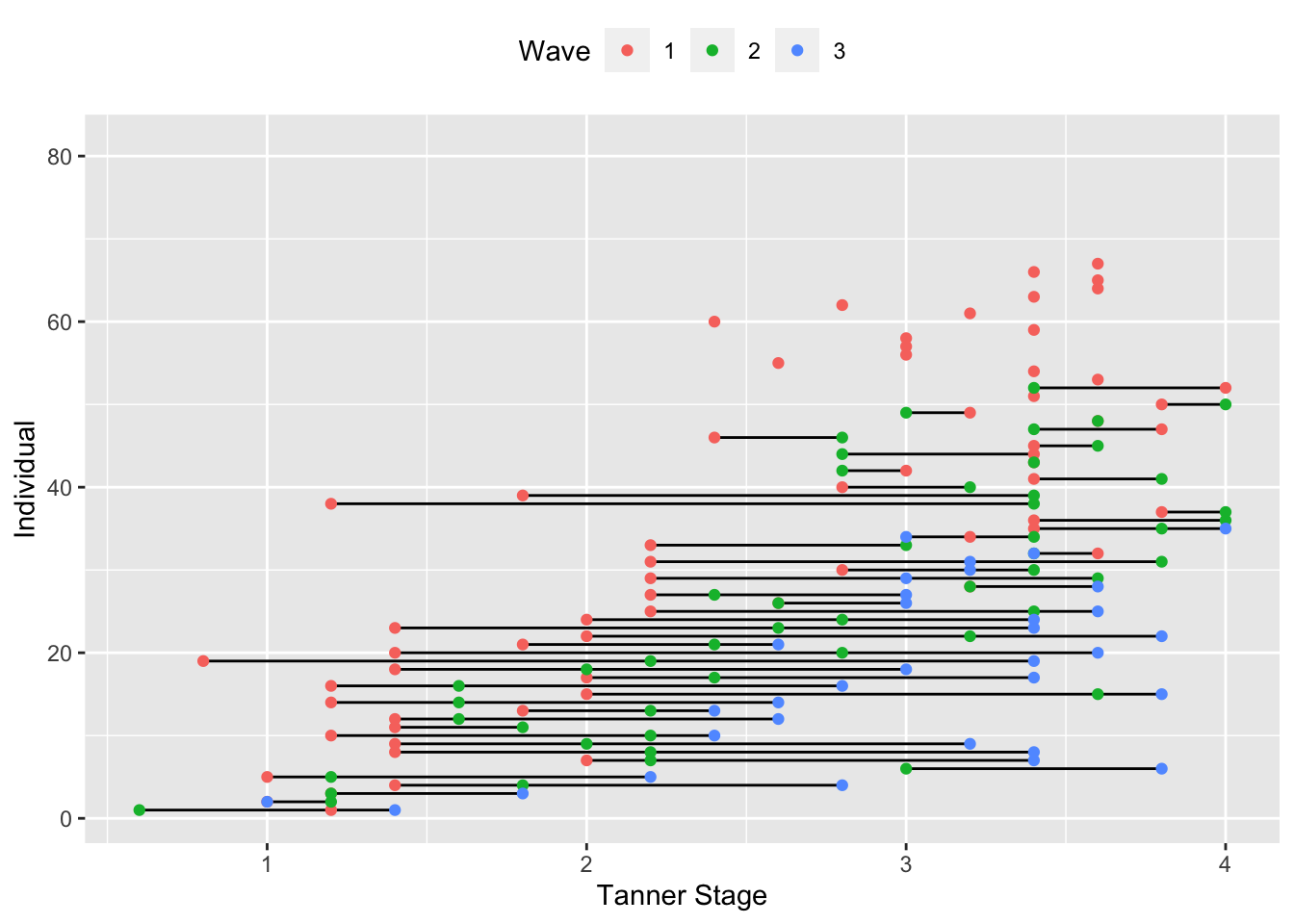
In some ways, this roughly resembles the age plot, with some individuals being measured at earlier stages of puberty and other later. However, close inspection starts to uncover some issues. First, we often stop measuring puberty once individual reach a certain age/stage of development, so puberty as a measure of maturation is limited in it’s utility outside of a fairly specific phase of development. We can already see for subjects who are measured first at later ages having missing data for later observations because puberty measures were not taken. There is also the curious case that some subset of individuals seem to move backwards in pubertal development (this should be treated as an error, but it’s amusing nonetheless). However, the key feature of interest in a plot like this is that, unlike age, there is not reason to expect that all individuals “age” at the same rate across puberty, seen by the uneven spacing between waves within individuals. This variation is just one of the exciting opportunities that modeling maturation using metric other than age present (although they do come with their own challenges; there is an admittedly understandable reason that age is the predominate variable in longitudinal models). One other advantage is within-age heterogeneity, which we can see by plotting Tanner Stage by age in the plot below.
ggplot(accelerated, aes(x = age, y = puberty)) +
  geom_line(aes(group = id), size = .5) +
  geom_point(aes(color = as.factor(wave))) +
  labs(x = "Age", y = "Tanner Stage", color = "Wave", shape = "Cohort") +
  theme(legend.position = "top")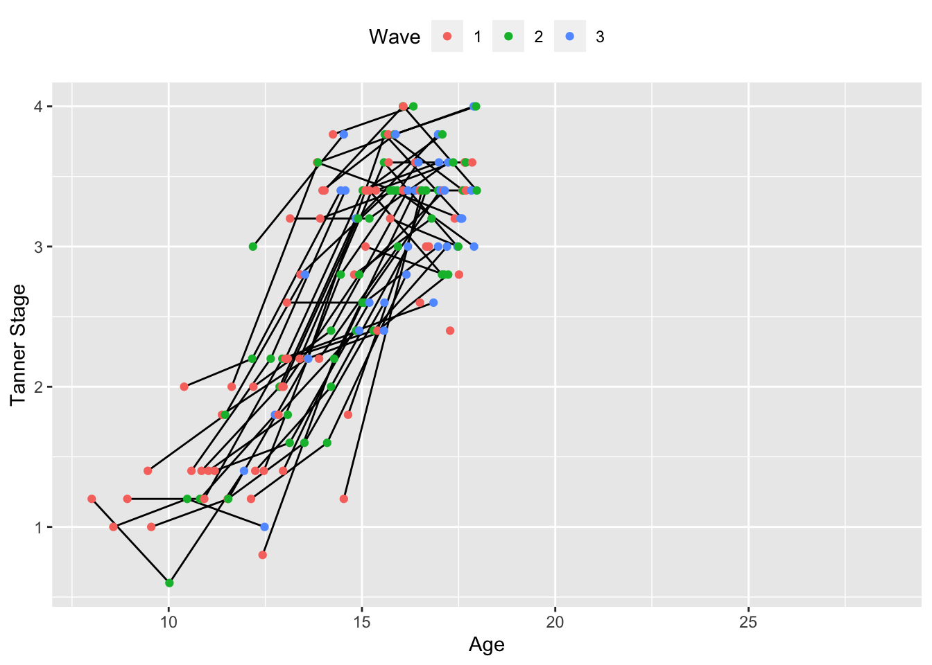
We can see that same-age peers may differ considerable (depending on when we measure them) in their pubertal development. We can also fit puberty-related trajectories to the modularity data below.
accel <- lmer(scale(modularity) ~ 1 + puberty + (1 | id),
              na.action = na.omit,
              REML = TRUE,
              data = accelerated)

summary(accel, correlation = FALSE)
## Linear mixed model fit by REML. t-tests use Satterthwaite's method [
## lmerModLmerTest]
## Formula: scale(modularity) ~ 1 + puberty + (1 | id)
## Data: accelerated
##
## REML criterion at convergence: 417.9
##
## Scaled residuals:
## Min 1Q Median 3Q Max
## -2.49262 -0.65415 0.04191 0.58260 2.43878
##
## Random effects:
## Groups Name Variance Std.Dev.
## id (Intercept) 0.3322 0.5763
## Residual 0.6698 0.8184
## Number of obs: 150, groups: id, 67
##
## Fixed effects:
## Estimate Std. Error df t value Pr(>|t|)
## (Intercept) -0.96653 0.28495 133.98649 -3.392 0.000913 ***
## puberty 0.34156 0.09681 145.04845 3.528 0.000561 ***
## ---
## Signif. codes: 0 '***' 0.001 '**' 0.01 '*' 0.05 '.' 0.1 ' ' 1Of course, we might wish to model age and puberty simultaneously. That may present practical challenges in this data, since age and puberty are highly correlated \(r = 0.796\), but some strategies for modeling multiple growth processes have been suggested elsewhere (see the relevant portion of the main text for details).
Residual Estimates
The final consideration we will explore in our discussion of time is the structure of the residuals of our repeated measures. This is often not of great theoretical importance (I don’t really believe you if you tell me your theory is specific enough to know if residual variance should be constant or not…call me a grinch), but it can be really important for model results. Essentially, an overly restrictive assumption about residual variances at the individual observation level can radiate out into the random effects structure and bias your effects. Here we will show how to specify both forms of a model in a mixed effect and structural equation model, and test which one is a better fit to the data.
We can start with the LCM, where heteroscedasticity (i.e., unique residual estimates across) is the default. To obtain this model, we use the same syntax we have seen repeatedly so far.
lcm.het <- "int =~ 1*dlpfc1 + 1*dlpfc2 + 1*dlpfc3 + 1*dlpfc4
            slp =~ 0*dlpfc1 + 1*dlpfc2 + 2*dlpfc3 + 3*dlpfc4"

lcm.het.fit <- growth(lcm.het,
                      data = single.cohort,
                      estimator = "ML",
                      missing = "FIML")

summary(lcm.het.fit, fit.measures = FALSE, estimates = TRUE,
        standardize = FALSE, rsquare = FALSE)
## lavaan 0.6.13 ended normally after 22 iterations
##
## Estimator ML
## Optimization method NLMINB
## Number of model parameters 9
##
## Number of observations 50
## Number of missing patterns 5
##
## Model Test User Model:
##
## Test statistic 12.140
## Degrees of freedom 5
## P-value (Chi-square) 0.033
##
## Parameter Estimates:
##
## Standard errors Standard
## Information Observed
## Observed information based on Hessian
##
## Latent Variables:
## Estimate Std.Err z-value P(>|z|)
## int =~
## dlpfc1 1.000
## dlpfc2 1.000
## dlpfc3 1.000
## dlpfc4 1.000
## slp =~
## dlpfc1 0.000
## dlpfc2 1.000
## dlpfc3 2.000
## dlpfc4 3.000
##
## Covariances:
## Estimate Std.Err z-value P(>|z|)
## int ~~
## slp -0.045 0.097 -0.467 0.641
##
## Intercepts:
## Estimate Std.Err z-value P(>|z|)
## .dlpfc1 0.000
## .dlpfc2 0.000
## .dlpfc3 0.000
## .dlpfc4 0.000
## int 0.628 0.132 4.761 0.000
## slp 0.114 0.054 2.120 0.034
##
## Variances:
## Estimate Std.Err z-value P(>|z|)
## .dlpfc1 0.280 0.196 1.427 0.154
## .dlpfc2 0.459 0.140 3.275 0.001
## .dlpfc3 0.389 0.128 3.039 0.002
## .dlpfc4 0.640 0.278 2.302 0.021
## int 0.631 0.207 3.039 0.002
## slp 0.055 0.054 1.010 0.313We can easily see that each residual obtains a unique value with an associated inference test (.dlpfc1 - .dlpfc4). To constrain these residuals equal across time, we have to explicitly write out the residual term (we have been relying on sensible defaults thus far) and then pre-multiply each estimate by the same alpha-numeric label. Lavaan will interpret repeated labels as a request for an equality constraint on those parameters. We can see this constraint in action below.
lcm.hom <- "int =~ 1*dlpfc1 + 1*dlpfc2 + 1*dlpfc3 + 1*dlpfc4
            slp =~ 0*dlpfc1 + 1*dlpfc2 + 2*dlpfc3 + 3*dlpfc4

            dlpfc1 ~~ c1*dlpfc1
            dlpfc2 ~~ c1*dlpfc2
            dlpfc3 ~~ c1*dlpfc3
            dlpfc4 ~~ c1*dlpfc4"
The choice of constraint (here c1) is somewhat arbitrary, but the point is that it can contain characters and numbers (although it must begin with a character). When we fit the model, we will see those parameters will be held equal.
lcm.hom.fit <- growth(lcm.hom,
                      data = single.cohort,
                      estimator = "ML",
                      missing = "FIML")

summary(lcm.hom.fit, fit.measures = FALSE, estimates = TRUE,
        standardize = FALSE, rsquare = FALSE)
## lavaan 0.6.13 ended normally after 19 iterations
##
## Estimator ML
## Optimization method NLMINB
## Number of model parameters 9
## Number of equality constraints 3
##
## Number of observations 50
## Number of missing patterns 5
##
## Model Test User Model:
##
## Test statistic 14.724
## Degrees of freedom 8
## P-value (Chi-square) 0.065
##
## Parameter Estimates:
##
## Standard errors Standard
## Information Observed
## Observed information based on Hessian
##
## Latent Variables:
## Estimate Std.Err z-value P(>|z|)
## int =~
## dlpfc1 1.000
## dlpfc2 1.000
## dlpfc3 1.000
## dlpfc4 1.000
## slp =~
## dlpfc1 0.000
## dlpfc2 1.000
## dlpfc3 2.000
## dlpfc4 3.000
##
## Covariances:
## Estimate Std.Err z-value P(>|z|)
## int ~~
## slp -0.041 0.061 -0.668 0.504
##
## Intercepts:
## Estimate Std.Err z-value P(>|z|)
## .dlpfc1 0.000
## .dlpfc2 0.000
## .dlpfc3 0.000
## .dlpfc4 0.000
## int 0.640 0.134 4.761 0.000
## slp 0.108 0.055 1.969 0.049
##
## Variances:
## Estimate Std.Err z-value P(>|z|)
## .dlpfc1 (c1) 0.435 0.065 6.732 0.000
## .dlpfc2 (c1) 0.435 0.065 6.732 0.000
## .dlpfc3 (c1) 0.435 0.065 6.732 0.000
## .dlpfc4 (c1) 0.435 0.065 6.732 0.000
## int 0.590 0.189 3.129 0.002
## slp 0.059 0.032 1.838 0.066Lavaan conveniently includes the labels in the output and we can see that now all of the residuals obtain the exact same value, and exact same inferential test (note how that changes the inference on the residual of dlpfc1 from above). However, note how other parameter estimates (namely the factor means and variances) change as well. These changes are small (for reasons we will see) but it is important to note we are making real changes to the model with the introduction of this constraint. We can then get a likelihood-ratio test of difference in fit, using the lavTestLRT() function, because the simplified homoscedastic model is nested within the more complex heteroscedastic model. Note that we list the homoscedastic model first.
lavaan::lavTestLRT(lcm.hom.fit, lcm.het.fit)##
## Chi-Squared Difference Test
##
## Df AIC BIC Chisq Chisq diff RMSEA Df diff Pr(>Chisq)
## lcm.het.fit 5 514.35 531.56 12.140
## lcm.hom.fit 8 510.93 522.40 14.724 2.5837 0 3 0.4604However, in the output, the heteroscedastic model is listed first. This is because the more complex model is always the reference and we are testing whether the imposition of model simplifications (i.e., constraints; here homoscedastic residuals) significantly decreases model fit. Here we can see that the chi-square difference test is not significant (\(p = 0.460\)), so we could retain the simplification without decreasing the fit of the model to our data. This is the reason that our parameters did not change much. In models where we would reject homoscedasticity, the imposition of the constraint would lead to more pronounced parameter changes elsewhere in the model. While there is not an associated inference test for the AIC/BIC, we could also use those values for model comparisons if we wished.
To implement heteroscedastic residuals in mixed-effects models, we have to leave our familiar lmer() and travel back in time to the days of lme(). We can first fit the canonical model we know and love, where the default is homoscedasticity.
mlm.hom <- nlme::lme(dlpfc ~ 1 + wave,
                     random = ~ 1 + wave | id,
                     na.action = na.omit,
                     method = "REML",
                     data = single.cohort.long)

summary(mlm.hom, correlation = FALSE)
## Linear mixed-effects model fit by REML
## Data: single.cohort.long
## AIC BIC logLik
## 517.3124 536.7629 -252.6562
##
## Random effects:
## Formula: ~1 + wave | id
## Structure: General positive-definite, Log-Cholesky parametrization
## StdDev Corr
## (Intercept) 0.8717474 (Intr)
## wave 0.2500535 -0.489
## Residual 0.6595289
##
## Fixed effects: dlpfc ~ 1 + wave
## Value Std.Error DF t-value p-value
## (Intercept) 0.5321058 0.16886967 140 3.150985 0.0020
## wave 0.1076007 0.05524678 140 1.947638 0.0535
## Correlation:
## (Intr)
## wave -0.705
##
## Standardized Within-Group Residuals:
## Min Q1 Med Q3 Max
## -2.09037990 -0.49924910 -0.04034052 0.65971936 2.07352349
##
## Number of Observations: 191
## Number of Groups: 50Note that in the Random effects portion of the output, we obtain a single numerical value for the residual \(\sigma^2 = 0.660\). To fit a heteroscedastic model, we need to make use of a new argument, weights. We can specify the form argument of the varIdent() (“variance identity) function to obtain a unique estimate per wave.
mlm.het <- nlme::lme(dlpfc ~ 1 + wave,
                     random = ~ 1 + wave | id,
                     weights = varIdent(form = ~ 1 | wave),
                     na.action = na.omit,
                     method = "REML",
                     data = single.cohort.long)

summary(mlm.het, correlation = FALSE)
## Linear mixed-effects model fit by REML
## Data: single.cohort.long
## AIC BIC logLik
## 520.7754 549.9511 -251.3877
##
## Random effects:
## Formula: ~1 + wave | id
## Structure: General positive-definite, Log-Cholesky parametrization
## StdDev Corr
## (Intercept) 0.8975009 (Intr)
## wave 0.2413003 -0.495
## Residual 0.5269518
##
## Variance function:
## Structure: Different standard deviations per stratum
## Formula: ~1 | wave
## Parameter estimates:
## 1 2 3 4
## 1.000000 1.287069 1.184203 1.515231
## Fixed effects: dlpfc ~ 1 + wave
## Value Std.Error DF t-value p-value
## (Intercept) 0.5144231 0.16258045 140 3.164114 0.0019
## wave 0.1139612 0.05386346 140 2.115743 0.0361
## Correlation:
## (Intr)
## wave -0.675
##
## Standardized Within-Group Residuals:
## Min Q1 Med Q3 Max
## -2.09852285 -0.47236320 -0.01588848 0.64203216 2.12263672
##
## Number of Observations: 191
## Number of Groups: 50Looking at the Random effects output, we still only see a single value for the residual. Unfortunately the output structure here leaves something to be desired. We need to look to the Variance function output section where we see for unique values. Well these are not technically the residual estimates, but rather they indicate the relative size of the residual scaled to the first estimate (the one we see in the Random effects section). To extract the actual estimates, we can use the following code.
mlm.het$sigma * exp(as.numeric(mlm.het$modelStruct$varStruct))## [1] 0.6782232 0.6240178 0.7984535So the first residual can be extracted as model$sigma, but the residual weights from the model are stuck in the varStruct portion of the fitted lme() object and are in the \(log(\sigma)\) scale. So we have to extract the values, convert them to numeric format, exponentiate them, and then multiple the weights by the estimated residual to obtain the other three estimates (tired yet?).
Fortunately, model comparisons are straightforward with the anova() function, which we can use in the same way we used lavTestLRT() to compare LCMs early.
anova(mlm.het, mlm.hom)## Model df AIC BIC logLik Test L.Ratio p-value
## mlm.het 1 9 520.7754 549.9511 -251.3877
## mlm.hom 2 6 517.3124 536.7629 -252.6562 1 vs 2 2.537015 0.4686Like before, these results indicate that imposing homoscedasticity does not significantly decrease model fit.