The Shape of Development
However, we define the underlying metric of time to structure our longitudinal model, one of the key substantive questions often underlying work in developmental science is to characterize the course that a given construct takes over time. Here we will highlight many of the different developmental trajectories that we can fit to our data, starting with relatively simple polynomial shapes and working our way up to modeling fully nonlinear trends. In addition to the feedback.learning data we have used thus far, we will also use data drawn from the external-math.csv and adversity.csv files. The external.math data contains up to \(5\) repeated observations from \(405\) children aged \(6\) to \(14\), measured once every \(2\) years. Here we will focus on measures of externalizing behavior and math proficiency. The adversity data contains fractional anisotropy (FA) measures from \(398\) children measured up to \(4\) times across ages \(4\) to \(11\). We previously used a subset of this data in the Time chapter, but here we will utilize the entire sample.
external.math <- read.csv("data/external-math.csv")

adversity <- read.csv("data/adversity.csv")

feedback.learning <- read.csv("data/feedback-learning.csv") %>%
  select(id, age, modularity, learning.rate)
Polynomial Trajectories
Like we discussed in the main text, polynomial trajectories are far and away the most common trajectories modeled with longitudinal data. They require relatively few unique timepoints, are straightforward to model, and offer easily-interpretable parameter estimates.
Intercept-Only Model
We can first consider the simplest polynomial model, one without even a slope. The intercept-only model simply models person-specific differences in average level across time. We can start here with the LCM, which makes the various specifications easiest to see, but we will also build syntax for models in the other frameworks.
int.lcm <- "int =~ 1*ext6 + 1*ext8 + 1*ext10 + 1*ext12 + 1*ext14"

int.lcm.fit <- growth(int.lcm,
                      data = external.math,
                      estimator = "ML",
                      missing = "FIML")

summary(int.lcm.fit, fit.measures = FALSE, estimates = TRUE,
        standardize = FALSE, rsquare = FALSE)
## lavaan 0.6.13 ended normally after 25 iterations
##
## Estimator ML
## Optimization method NLMINB
## Number of model parameters 7
##
## Number of observations 405
## Number of missing patterns 21
##
## Model Test User Model:
##
## Test statistic 71.246
## Degrees of freedom 13
## P-value (Chi-square) 0.000
##
## Parameter Estimates:
##
## Standard errors Standard
## Information Observed
## Observed information based on Hessian
##
## Latent Variables:
## Estimate Std.Err z-value P(>|z|)
## int =~
## ext6 1.000
## ext8 1.000
## ext10 1.000
## ext12 1.000
## ext14 1.000
##
## Intercepts:
## Estimate Std.Err z-value P(>|z|)
## .ext6 0.000
## .ext8 0.000
## .ext10 0.000
## .ext12 0.000
## .ext14 0.000
## int 1.882 0.077 24.397 0.000
##
## Variances:
## Estimate Std.Err z-value P(>|z|)
## .ext6 1.761 0.203 8.690 0.000
## .ext8 1.771 0.189 9.384 0.000
## .ext10 2.023 0.208 9.730 0.000
## .ext12 2.243 0.230 9.758 0.000
## .ext14 2.049 0.348 5.891 0.000
## int 1.752 0.172 10.161 0.000We can see that there is significant variance in the intercept factor, suggesting meaningful person-to-person variability in level of externalizing behavior during late childhood and early adolescence. While this might seem a somewhat silly model to fit to these data, this is one half of a random-intercept cross-lag panel model and might be appropriate if we do not expect systematic change over time. However, these intercept-only models are admittedly more plausible for intensive longitudinal data. The MLM specification for this model can be seen below. We will first transform the data into long format before fitting the model.
external.math.long <- external.math %>%
  pivot_longer(cols = starts_with(c("ext", "math")),
                      names_to = c(".value", "age"),
                      names_pattern = "(ext|math)(.+)") %>%
  mutate(age = as.numeric(age))

int.mlm <- lmer(ext ~ 1 + (1 | id),
                na.action = na.omit,
                REML = TRUE,
                data = external.math.long)

summary(int.mlm, correlation = FALSE)
## Linear mixed model fit by REML. t-tests use Satterthwaite's method [
## lmerModLmerTest]
## Formula: ext ~ 1 + (1 | id)
## Data: external.math.long
##
## REML criterion at convergence: 5316.7
##
## Scaled residuals:
## Min 1Q Median 3Q Max
## -3.2539 -0.5600 -0.2063 0.4736 4.5276
##
## Random effects:
## Groups Name Variance Std.Dev.
## id (Intercept) 1.799 1.341
## Residual 1.944 1.394
## Number of obs: 1357, groups: id, 405
##
## Fixed effects:
## Estimate Std. Error df t value Pr(>|t|)
## (Intercept) 1.89455 0.07736 399.24978 24.49 <2e-16 ***
## ---
## Signif. codes: 0 '***' 0.001 '**' 0.01 '*' 0.05 '.' 0.1 ' ' 1Note that this is just a random-effects ANOVA model with no predictors.
Linear Model
We will move quickly through the linear polynomial models because we have covered them extensively thus far. Below is the syntax for the linear LCM. Remember that assessments are biannual so factor loadings should increase by two for each wave.
lin.lcm <- "int =~ 1*ext6 + 1*ext8 + 1*ext10 + 1*ext12 + 1*ext14
            slp =~ 0*ext6 + 2*ext8 + 4*ext10 + 6*ext12 + 8*ext14"

lin.lcm.fit <- growth(lin.lcm,
                      data = external.math,
                      estimator = "ML",
                      missing = "FIML")

summary(lin.lcm.fit, fit.measures = FALSE, estimates = TRUE,
        standardize = FALSE, rsquare = FALSE)
## lavaan 0.6.13 ended normally after 36 iterations
##
## Estimator ML
## Optimization method NLMINB
## Number of model parameters 10
##
## Number of observations 405
## Number of missing patterns 21
##
## Model Test User Model:
##
## Test statistic 19.507
## Degrees of freedom 10
## P-value (Chi-square) 0.034
##
## Parameter Estimates:
##
## Standard errors Standard
## Information Observed
## Observed information based on Hessian
##
## Latent Variables:
## Estimate Std.Err z-value P(>|z|)
## int =~
## ext6 1.000
## ext8 1.000
## ext10 1.000
## ext12 1.000
## ext14 1.000
## slp =~
## ext6 0.000
## ext8 2.000
## ext10 4.000
## ext12 6.000
## ext14 8.000
##
## Covariances:
## Estimate Std.Err z-value P(>|z|)
## int ~~
## slp 0.084 0.042 2.003 0.045
##
## Intercepts:
## Estimate Std.Err z-value P(>|z|)
## .ext6 0.000
## .ext8 0.000
## .ext10 0.000
## .ext12 0.000
## .ext14 0.000
## int 1.664 0.081 20.459 0.000
## slp 0.074 0.018 4.135 0.000
##
## Variances:
## Estimate Std.Err z-value P(>|z|)
## .ext6 1.653 0.239 6.914 0.000
## .ext8 1.844 0.188 9.807 0.000
## .ext10 1.910 0.199 9.593 0.000
## .ext12 1.592 0.227 7.007 0.000
## .ext14 1.618 0.372 4.346 0.000
## int 1.068 0.227 4.710 0.000
## slp 0.024 0.011 2.066 0.039While we have ignored model fit for most models, one nice thing about many of these models, is that they are nested and allow for formal model comparison with likelihood ratio tests, similar to those we saw with hetero- vs. homoscedastic residuals. For instance, we can compare the intercept-only with a linear model.
lavTestLRT(int.lcm.fit, lin.lcm.fit)##
## Chi-Squared Difference Test
##
## Df AIC BIC Chisq Chisq diff RMSEA Df diff Pr(>Chisq)
## lin.lcm.fit 10 5278.2 5318.3 19.506
## int.lcm.fit 13 5324.0 5352.0 71.246 51.74 0.20029 3 3.403e-11 ***
## ---
## Signif. codes: 0 '***' 0.001 '**' 0.01 '*' 0.05 '.' 0.1 ' ' 1Remember that we compare whether the more constrained model (here the intercept-only) induces a significant decrease in model fit. Here this is true, suggesting that we should retain the linear model over the intercept-only model. If we take a peak at the model fit, this is because the linear model fits the data reasonably well, while the intercept-only model is quite poor in terms of fit.
summary(int.lcm.fit, fit.measures = TRUE, estimates = FALSE,
        standardize = FALSE, rsquare = FALSE)
## lavaan 0.6.13 ended normally after 25 iterations
##
## Estimator ML
## Optimization method NLMINB
## Number of model parameters 7
##
## Number of observations 405
## Number of missing patterns 21
##
## Model Test User Model:
##
## Test statistic 71.246
## Degrees of freedom 13
## P-value (Chi-square) 0.000
##
## Model Test Baseline Model:
##
## Test statistic 361.048
## Degrees of freedom 10
## P-value 0.000
##
## User Model versus Baseline Model:
##
## Comparative Fit Index (CFI) 0.834
## Tucker-Lewis Index (TLI) 0.872
##
## Robust Comparative Fit Index (CFI) 0.854
## Robust Tucker-Lewis Index (TLI) 0.888
##
## Loglikelihood and Information Criteria:
##
## Loglikelihood user model (H0) -2654.990
## Loglikelihood unrestricted model (H1) -2619.367
##
## Akaike (AIC) 5323.980
## Bayesian (BIC) 5352.007
## Sample-size adjusted Bayesian (SABIC) 5329.795
##
## Root Mean Square Error of Approximation:
##
## RMSEA 0.105
## 90 Percent confidence interval - lower 0.082
## 90 Percent confidence interval - upper 0.130
## P-value H_0: RMSEA <= 0.050 0.000
## P-value H_0: RMSEA >= 0.080 0.963
##
## Robust RMSEA 0.144
## 90 Percent confidence interval - lower 0.099
## 90 Percent confidence interval - upper 0.191
## P-value H_0: Robust RMSEA <= 0.050 0.001
## P-value H_0: Robust RMSEA >= 0.080 0.989
##
## Standardized Root Mean Square Residual:
##
## SRMR 0.156summary(lin.lcm.fit, fit.measures = TRUE, estimates = FALSE,
standardize = FALSE, rsquare = FALSE)## lavaan 0.6.13 ended normally after 36 iterations
##
## Estimator ML
## Optimization method NLMINB
## Number of model parameters 10
##
## Number of observations 405
## Number of missing patterns 21
##
## Model Test User Model:
##
## Test statistic 19.507
## Degrees of freedom 10
## P-value (Chi-square) 0.034
##
## Model Test Baseline Model:
##
## Test statistic 361.048
## Degrees of freedom 10
## P-value 0.000
##
## User Model versus Baseline Model:
##
## Comparative Fit Index (CFI) 0.973
## Tucker-Lewis Index (TLI) 0.973
##
## Robust Comparative Fit Index (CFI) 0.946
## Robust Tucker-Lewis Index (TLI) 0.946
##
## Loglikelihood and Information Criteria:
##
## Loglikelihood user model (H0) -2629.120
## Loglikelihood unrestricted model (H1) -2619.367
##
## Akaike (AIC) 5278.240
## Bayesian (BIC) 5318.279
## Sample-size adjusted Bayesian (SABIC) 5286.547
##
## Root Mean Square Error of Approximation:
##
## RMSEA 0.048
## 90 Percent confidence interval - lower 0.013
## 90 Percent confidence interval - upper 0.080
## P-value H_0: RMSEA <= 0.050 0.486
## P-value H_0: RMSEA >= 0.080 0.052
##
## Robust RMSEA 0.100
## 90 Percent confidence interval - lower 0.042
## 90 Percent confidence interval - upper 0.157
## P-value H_0: Robust RMSEA <= 0.050 0.072
## P-value H_0: Robust RMSEA >= 0.080 0.753
##
## Standardized Root Mean Square Residual:
##
## SRMR 0.082To fit the corresponding MLM, we first need to generate our linear predictor as an observed variable in our data frame (and will need to do so each time we increase the order of the model). Here we will generate the linear predictor by simply subtracting \(6\) from the age variable.
external.math.long$age <- external.math.long$age - min(external.math.long$age)

lin.mlm <- lmer(ext ~ 1 + age + (1 + age | id),
                na.action = na.omit,
                REML = TRUE,
                data = external.math.long,
                control = lmerControl(optimizer = "bobyqa",
                                      optCtrl = list(maxfun = 2e5)))

summary(lin.mlm, correlation = FALSE)
## Linear mixed model fit by REML. t-tests use Satterthwaite's method [
## lmerModLmerTest]
## Formula: ext ~ 1 + age + (1 + age | id)
## Data: external.math.long
## Control: lmerControl(optimizer = "bobyqa", optCtrl = list(maxfun = 2e+05))
##
## REML criterion at convergence: 5269.3
##
## Scaled residuals:
## Min 1Q Median 3Q Max
## -3.1375 -0.5422 -0.1737 0.4491 3.9389
##
## Random effects:
## Groups Name Variance Std.Dev. Corr
## id (Intercept) 1.02975 1.0148
## age 0.01778 0.1334 0.75
## Residual 1.78241 1.3351
## Number of obs: 1357, groups: id, 405
##
## Fixed effects:
## Estimate Std. Error df t value Pr(>|t|)
## (Intercept) 1.66939 0.08114 372.83468 20.574 < 2e-16 ***
## age 0.07235 0.01758 288.52536 4.116 5.03e-05 ***
## ---
## Signif. codes: 0 '***' 0.001 '**' 0.01 '*' 0.05 '.' 0.1 ' ' 1And the model comparison reveals the same preference for the linear model. Note that the model is re-estimated with ML [FIML] because the two models contain different fixed effects. REML models can be compared when the models differ only in the variance structure. Fortunately this will be done automatically so we don’t have to “manually” re-estimate the models.
anova(int.mlm, lin.mlm)## Data: external.math.long
## Models:
## int.mlm: ext ~ 1 + (1 | id)
## lin.mlm: ext ~ 1 + age + (1 + age | id)
## npar AIC BIC logLik deviance Chisq Df Pr(>Chisq)
## int.mlm 3 5319.5 5335.1 -2656.7 5313.5
## lin.mlm 6 5271.7 5303.0 -2629.9 5259.7 53.736 3 1.277e-11 ***
## ---
## Signif. codes: 0 '***' 0.001 '**' 0.01 '*' 0.05 '.' 0.1 ' ' 1Finally, we can see a version of the linear LCSM for the external.math data below. Note again that biannual observations mean that we need to set the factor loadings for the slope factor to \(2\) instead of \(1\) to indicate the spacing appropriately.
lin.lcsm <- "
            # Define Phantom Variables (p = phantom)
            pext6 =~ 1*ext6; ext6 ~ 0; ext6 ~~ ext6; pext6 ~~ 0*pext6
            pext8 =~ 1*ext8; ext8 ~ 0; ext8 ~~ ext8; pext8 ~~ 0*pext8
            pext10 =~ 1*ext10; ext10 ~ 0; ext10 ~~ ext10; pext10 ~~ 0*pext10
            pext12 =~ 1*ext12; ext12 ~ 0; ext12 ~~ ext12; pext12 ~~ 0*pext12
            pext14 =~ 1*ext14; ext14 ~ 0; ext14 ~~ ext14; pext14 ~~ 0*pext14

            # Regressions Between Adjacent Observations
            pext8 ~ 1*pext6
            pext10 ~ 1*pext8
            pext12 ~ 1*pext10
            pext14 ~ 1*pext12

            # Define Change Latent Variables (delta)
            delta21 =~ 1*pext8;  delta21 ~~ 0*delta21
            delta32 =~ 1*pext10; delta32 ~~ 0*delta32
            delta43 =~ 1*pext12; delta43 ~~ 0*delta43
            delta54 =~ 1*pext14; delta54 ~~ 0*delta54

            # Define Intercept and Slope
            int =~ 1*pext6
            slp =~ 2*delta21 + 2*delta32 + 2*delta43 + 2*delta54

            int ~ 1
            slp ~ 1

            int ~~ slp
            slp ~~ slp
"

lin.lcsm.fit <- sem(lin.lcsm,
                    data = external.math,
                    estimator = "ML",
                    missing = "FIML")

summary(lin.lcsm.fit, fit.measures = FALSE, estimates = TRUE,
        standardize = FALSE, rsquare = FALSE)
## lavaan 0.6.13 ended normally after 36 iterations
##
## Estimator ML
## Optimization method NLMINB
## Number of model parameters 10
##
## Number of observations 405
## Number of missing patterns 21
##
## Model Test User Model:
##
## Test statistic 19.507
## Degrees of freedom 10
## P-value (Chi-square) 0.034
##
## Parameter Estimates:
##
## Standard errors Standard
## Information Observed
## Observed information based on Hessian
##
## Latent Variables:
## Estimate Std.Err z-value P(>|z|)
## pext6 =~
## ext6 1.000
## pext8 =~
## ext8 1.000
## pext10 =~
## ext10 1.000
## pext12 =~
## ext12 1.000
## pext14 =~
## ext14 1.000
## delta21 =~
## pext8 1.000
## delta32 =~
## pext10 1.000
## delta43 =~
## pext12 1.000
## delta54 =~
## pext14 1.000
## int =~
## pext6 1.000
## slp =~
## delta21 2.000
## delta32 2.000
## delta43 2.000
## delta54 2.000
##
## Regressions:
## Estimate Std.Err z-value P(>|z|)
## pext8 ~
## pext6 1.000
## pext10 ~
## pext8 1.000
## pext12 ~
## pext10 1.000
## pext14 ~
## pext12 1.000
##
## Covariances:
## Estimate Std.Err z-value P(>|z|)
## int ~~
## slp 0.084 0.042 2.003 0.045
##
## Intercepts:
## Estimate Std.Err z-value P(>|z|)
## .ext6 0.000
## .ext8 0.000
## .ext10 0.000
## .ext12 0.000
## .ext14 0.000
## int 1.664 0.081 20.459 0.000
## slp 0.074 0.018 4.135 0.000
## .pext6 0.000
## .pext8 0.000
## .pext10 0.000
## .pext12 0.000
## .pext14 0.000
## .delta21 0.000
## .delta32 0.000
## .delta43 0.000
## .delta54 0.000
##
## Variances:
## Estimate Std.Err z-value P(>|z|)
## .ext6 1.653 0.239 6.914 0.000
## .pext6 0.000
## .ext8 1.844 0.188 9.807 0.000
## .pext8 0.000
## .ext10 1.910 0.199 9.593 0.000
## .pext10 0.000
## .ext12 1.592 0.227 7.007 0.000
## .pext12 0.000
## .ext14 1.618 0.372 4.346 0.000
## .pext14 0.000
## .delta21 0.000
## .delta32 0.000
## .delta43 0.000
## .delta54 0.000
## slp 0.024 0.011 2.066 0.039
## int 1.068 0.227 4.710 0.000Quadratic Model
Next, we can add an additional factor to capture quadratic curvature in our data. Below is the LCM syntax for this model. Note that this is an extremely straightforward expansion of the syntax we have seen thus far. While this won’t be the case here, sometimes we need to worry about numerically large factor loadings causing some estimation issues in practice (nothing theoretical is wrong with large factor loadings). In those instances, we could divide our factor loadings by some constant to control those values from getting to large (although this will change the interpretation of a per-unit change).
quad.lcm <- "int  =~ 1*ext6 + 1*ext8 + 1*ext10 + 1*ext12 + 1*ext14
             slp  =~ 0*ext6 + 2*ext8 + 4*ext10 + 6*ext12 + 8*ext14
             quad =~ 0*ext6 + 4*ext8 + 16*ext10 + 36*ext12 + 64*ext14"

quad.lcm.fit <- growth(quad.lcm,
                       data = external.math,
                       estimator = "ML",
                       missing = "FIML")

summary(quad.lcm.fit, fit.measures = FALSE, estimates = TRUE,
        standardize = TRUE, rsquare = FALSE)
## lavaan 0.6.13 ended normally after 95 iterations
##
## Estimator ML
## Optimization method NLMINB
## Number of model parameters 14
##
## Number of observations 405
## Number of missing patterns 21
##
## Model Test User Model:
##
## Test statistic 5.437
## Degrees of freedom 6
## P-value (Chi-square) 0.489
##
## Parameter Estimates:
##
## Standard errors Standard
## Information Observed
## Observed information based on Hessian
##
## Latent Variables:
## Estimate Std.Err z-value P(>|z|) Std.lv Std.all
## int =~
## ext6 1.000 1.166 0.731
## ext8 1.000 1.166 0.625
## ext10 1.000 1.166 0.566
## ext12 1.000 1.166 0.546
## ext14 1.000 1.166 0.551
## slp =~
## ext6 0.000 0.000 0.000
## ext8 2.000 1.040 0.558
## ext10 4.000 2.079 1.010
## ext12 6.000 3.119 1.461
## ext14 8.000 4.159 1.964
## quad =~
## ext6 0.000 0.000 0.000
## ext8 4.000 0.228 0.122
## ext10 16.000 0.912 0.443
## ext12 36.000 2.051 0.961
## ext14 64.000 3.647 1.722
##
## Covariances:
## Estimate Std.Err z-value P(>|z|) Std.lv Std.all
## int ~~
## slp -0.108 0.209 -0.514 0.607 -0.177 -0.177
## quad 0.018 0.023 0.772 0.440 0.270 0.270
## slp ~~
## quad -0.029 0.015 -1.933 0.053 -0.970 -0.970
##
## Intercepts:
## Estimate Std.Err z-value P(>|z|) Std.lv Std.all
## .ext6 0.000 0.000 0.000
## .ext8 0.000 0.000 0.000
## .ext10 0.000 0.000 0.000
## .ext12 0.000 0.000 0.000
## .ext14 0.000 0.000 0.000
## int 1.567 0.088 17.809 0.000 1.344 1.344
## slp 0.182 0.051 3.535 0.000 0.349 0.349
## quad -0.015 0.007 -2.300 0.021 -0.271 -0.271
##
## Variances:
## Estimate Std.Err z-value P(>|z|) Std.lv Std.all
## .ext6 1.188 0.431 2.758 0.006 1.188 0.466
## .ext8 1.731 0.191 9.076 0.000 1.731 0.498
## .ext10 1.691 0.215 7.858 0.000 1.691 0.399
## .ext12 1.672 0.227 7.379 0.000 1.672 0.367
## .ext14 1.381 0.649 2.128 0.033 1.381 0.308
## int 1.360 0.431 3.159 0.002 1.000 1.000
## slp 0.270 0.124 2.175 0.030 1.000 1.000
## quad 0.003 0.002 1.705 0.088 1.000 1.000lavTestLRT(lin.lcm.fit, quad.lcm.fit)##
## Chi-Squared Difference Test
##
## Df AIC BIC Chisq Chisq diff RMSEA Df diff Pr(>Chisq)
## quad.lcm.fit 6 5272.2 5328.2 5.4373
## lin.lcm.fit 10 5278.2 5318.3 19.5065 14.069 0.078839 4 0.007077 **
## ---
## Signif. codes: 0 '***' 0.001 '**' 0.01 '*' 0.05 '.' 0.1 ' ' 1The MLM syntax is similarly straightforward. To add a powered term, we can use the I() function, or the poly() function if we wished to use orthogonal polynomials.
quad.mlm <- lmer(ext ~ 1 + age + I(age^2) + (1 + age + I(age^2) | id),
                 na.action = na.omit,
                 REML = TRUE,
                 data = external.math.long,
                 control = lmerControl(optimizer = "bobyqa",
                                       optCtrl = list(maxfun = 2e5)))

summary(quad.mlm, correlation = FALSE)
## Linear mixed model fit by REML. t-tests use Satterthwaite's method [
## lmerModLmerTest]
## Formula: ext ~ 1 + age + I(age^2) + (1 + age + I(age^2) | id)
## Data: external.math.long
## Control: lmerControl(optimizer = "bobyqa", optCtrl = list(maxfun = 2e+05))
##
## REML criterion at convergence: 5263.6
##
## Scaled residuals:
## Min 1Q Median 3Q Max
## -3.2948 -0.5378 -0.1802 0.4328 4.1605
##
## Random effects:
## Groups Name Variance Std.Dev. Corr
## id (Intercept) 0.942787 0.97097
## age 0.162793 0.40348 0.27
## I(age^2) 0.001871 0.04325 -0.12 -0.96
## Residual 1.684821 1.29801
## Number of obs: 1357, groups: id, 405
##
## Fixed effects:
## Estimate Std. Error df t value Pr(>|t|)
## (Intercept) 1.574442 0.087961 345.809227 17.899 < 2e-16 ***
## age 0.178331 0.051186 357.020201 3.484 0.000555 ***
## I(age^2) -0.015107 0.006678 299.946299 -2.262 0.024398 *
## ---
## Signif. codes: 0 '***' 0.001 '**' 0.01 '*' 0.05 '.' 0.1 ' ' 1While these models converge without too much issue here, note the strong correlation between the linear and quadratic terms, suggesting that the quadratic term is largely redundant. This is often the case with low numbers of repeated measures. We can technically fit some non-linearities, but they may not be particularly well-specified.
The LCSM syntax requires a bit more explanation. The quadratic model is shown below.
quad.lcsm <- "
             # Define Phantom Variables (p = phantom)
             pext6 =~ 1*ext6; ext6 ~ 0; ext6 ~~ ext6; pext6 ~~ 0*pext6
             pext8 =~ 1*ext8; ext8 ~ 0; ext8 ~~ ext8; pext8 ~~ 0*pext8
             pext10 =~ 1*ext10; ext10 ~ 0; ext10 ~~ ext10; pext10 ~~ 0*pext10
             pext12 =~ 1*ext12; ext12 ~ 0; ext12 ~~ ext12; pext12 ~~ 0*pext12
             pext14 =~ 1*ext14; ext14 ~ 0; ext14 ~~ ext14; pext14 ~~ 0*pext14

             # Regressions Between Adjacent Observations
             pext8 ~ 1*pext6
             pext10 ~ 1*pext8
             pext12 ~ 1*pext10
             pext14 ~ 1*pext12

             # Define Change Latent Variables (delta)
             delta21 =~ 1*pext8;  delta21 ~~ 0*delta21
             delta32 =~ 1*pext10; delta32 ~~ 0*delta32
             delta43 =~ 1*pext12; delta43 ~~ 0*delta43
             delta54 =~ 1*pext14; delta54 ~~ 0*delta54

             # Define Intercept and Slope
             int  =~ 1*pext6
             slp  =~ 2*delta21 + 2*delta32 + 2*delta43 + 2*delta54
             quad =~ 4*delta21 + 12*delta32 + 20*delta43 + 28*delta54

             int  ~ 1
             slp  ~ 1
             quad ~ 1

             int ~~ slp
             int ~~ quad
             slp ~~ slp
             slp ~~ quad
             quad ~~ quad
"
We talked in the Canonical chapter about how the loadings for the linear factor were all \(1\), and this could be thought of as summing across the difference factors. Another way to think of this specification is that the factor loadings for the LCSM are the differences between successive loadings for the LCM. In the standard linear case, these are all \(1\)s to indicate a constant effect across units of time, whereas in our example in this chapter, they are all differences of \(2\) to reflect biannual observations. The same principle can be applied to the loadings for higher-order factors in the LCSM. For a quadratic factor, the LCM loadings are [\(0\), \(4\), \(16\), \(36\), \(64\)], and therefore the LCSM loadings should be [(\(4 - 0\)), (\(16 - 4\)), (\(36 - 16\)), (\(64 - 36\))] = [\(4\), \(12\), \(20\), \(28\)]. As a sanity check, we can fit this model and the parameter estimates should match the LCM results exactly.
quad.lcsm.fit <- sem(quad.lcsm,
                     data = external.math,
                     estimator = "ML",
                     missing = "FIML")

summary(quad.lcsm.fit, fit.measures = FALSE, estimates = TRUE,
        standardize = TRUE, rsquare = FALSE)
## lavaan 0.6.13 ended normally after 95 iterations
##
## Estimator ML
## Optimization method NLMINB
## Number of model parameters 14
##
## Number of observations 405
## Number of missing patterns 21
##
## Model Test User Model:
##
## Test statistic 5.437
## Degrees of freedom 6
## P-value (Chi-square) 0.489
##
## Parameter Estimates:
##
## Standard errors Standard
## Information Observed
## Observed information based on Hessian
##
## Latent Variables:
## Estimate Std.Err z-value P(>|z|) Std.lv Std.all
## pext6 =~
## ext6 1.000 1.166 0.731
## pext8 =~
## ext8 1.000 1.322 0.709
## pext10 =~
## ext10 1.000 1.597 0.775
## pext12 =~
## ext12 1.000 1.698 0.796
## pext14 =~
## ext14 1.000 1.761 0.832
## delta21 =~
## pext8 1.000 0.621 0.621
## delta32 =~
## pext10 1.000 0.257 0.257
## delta43 =~
## pext12 1.000 0.167 0.167
## delta54 =~
## pext14 1.000 0.362 0.362
## int =~
## pext6 1.000 1.000 1.000
## slp =~
## delta21 2.000 1.267 1.267
## delta32 2.000 2.529 2.529
## delta43 2.000 3.665 3.665
## delta54 2.000 1.629 1.629
## quad =~
## delta21 4.000 0.278 0.278
## delta32 12.000 1.663 1.663
## delta43 20.000 4.017 4.017
## delta54 28.000 2.499 2.499
##
## Regressions:
## Estimate Std.Err z-value P(>|z|) Std.lv Std.all
## pext8 ~
## pext6 1.000 0.882 0.882
## pext10 ~
## pext8 1.000 0.828 0.828
## pext12 ~
## pext10 1.000 0.941 0.941
## pext14 ~
## pext12 1.000 0.964 0.964
##
## Covariances:
## Estimate Std.Err z-value P(>|z|) Std.lv Std.all
## int ~~
## slp -0.108 0.209 -0.514 0.607 -0.177 -0.177
## quad 0.018 0.023 0.772 0.440 0.270 0.270
## slp ~~
## quad -0.029 0.015 -1.933 0.053 -0.970 -0.970
##
## Intercepts:
## Estimate Std.Err z-value P(>|z|) Std.lv Std.all
## .ext6 0.000 0.000 0.000
## .ext8 0.000 0.000 0.000
## .ext10 0.000 0.000 0.000
## .ext12 0.000 0.000 0.000
## .ext14 0.000 0.000 0.000
## int 1.567 0.088 17.809 0.000 1.344 1.344
## slp 0.182 0.051 3.535 0.000 0.349 0.349
## quad -0.015 0.007 -2.300 0.021 -0.271 -0.271
## .pext6 0.000 0.000 0.000
## .pext8 0.000 0.000 0.000
## .pext10 0.000 0.000 0.000
## .pext12 0.000 0.000 0.000
## .pext14 0.000 0.000 0.000
## .delta21 0.000 0.000 0.000
## .delta32 0.000 0.000 0.000
## .delta43 0.000 0.000 0.000
## .delta54 0.000 0.000 0.000
##
## Variances:
## Estimate Std.Err z-value P(>|z|) Std.lv Std.all
## .ext6 1.188 0.431 2.758 0.006 1.188 0.466
## .pext6 0.000 0.000 0.000
## .ext8 1.731 0.191 9.076 0.000 1.731 0.498
## .pext8 0.000 0.000 0.000
## .ext10 1.691 0.215 7.858 0.000 1.691 0.399
## .pext10 0.000 0.000 0.000
## .ext12 1.672 0.227 7.379 0.000 1.672 0.367
## .pext12 0.000 0.000 0.000
## .ext14 1.381 0.649 2.128 0.033 1.381 0.308
## .pext14 0.000 0.000 0.000
## .delta21 0.000 0.000 0.000
## .delta32 0.000 0.000 0.000
## .delta43 0.000 0.000 0.000
## .delta54 0.000 0.000 0.000
## slp 0.270 0.124 2.175 0.030 1.000 1.000
## quad 0.003 0.002 1.705 0.088 1.000 1.000
## int 1.360 0.431 3.159 0.002 1.000 1.000lavTestLRT(lin.lcsm.fit, quad.lcsm.fit)##
## Chi-Squared Difference Test
##
## Df AIC BIC Chisq Chisq diff RMSEA Df diff Pr(>Chisq)
## quad.lcsm.fit 6 5272.2 5328.2 5.4373
## lin.lcsm.fit 10 5278.2 5318.3 19.5065 14.069 0.078839 4 0.007077
##
## quad.lcsm.fit
## lin.lcsm.fit **
## ---
## Signif. codes: 0 '***' 0.001 '**' 0.01 '*' 0.05 '.' 0.1 ' ' 1Inverse Model
The final polynomial model we will consider is the inverse model. Unlike the quadratic curvature which reverses, the inverse curve approaches a plateau asymptotically. We can do a quick algebraic transformation to make the factor loadings tractable by inverting the original (i.e., not centered) values and subtracting them from \(1\). So for linear loadings [\(1\), \(3\), \(5\), \(7\), \(9\)], we would have inverse factor loadings [\(1 - (1/1)\), \(1 - (1/3)\), \(1 - (1/5)\), \(1 - (1/7)\), \(1 - (1/9)\)] or [\(0\), \(2/3\), \(4/5\), \(6/7\), \(8/9\)]. Inverting the original loadings avoids trying to take the reciprocal of 0 (which results in 6 more weeks of COVID variants) and subtracting from one specifies an upper rather than lower bound effect (this won’t change the nature of the effect, it just makes the sign easier to interpret).
inv.lcm <- "int =~ 1*ext6 + 1*ext8 + 1*ext10 + 1*ext12 + 1*ext14
            slp =~ 0*ext6 + 2*ext8 + 4*ext10 + 6*ext12 + 8*ext14
            inv =~ 0*ext6 + (2/3)*ext8 + (4/5)*ext10 + (6/7)*ext12 + (7/8)*ext14"

inv.lcm.fit <- growth(inv.lcm,
                      data = external.math,
                      estimator = "ML",
                      missing = "FIML")

summary(inv.lcm.fit, fit.measures = FALSE, estimates = TRUE,
        standardize = TRUE, rsquare = FALSE)
## lavaan 0.6.13 ended normally after 64 iterations
##
## Estimator ML
## Optimization method NLMINB
## Number of model parameters 14
##
## Number of observations 405
## Number of missing patterns 21
##
## Model Test User Model:
##
## Test statistic 5.839
## Degrees of freedom 6
## P-value (Chi-square) 0.442
##
## Parameter Estimates:
##
## Standard errors Standard
## Information Observed
## Observed information based on Hessian
##
## Latent Variables:
## Estimate Std.Err z-value P(>|z|) Std.lv Std.all
## int =~
## ext6 1.000 1.747 1.099
## ext8 1.000 1.747 0.925
## ext10 1.000 1.747 0.855
## ext12 1.000 1.747 0.830
## ext14 1.000 1.747 0.799
## slp =~
## ext6 0.000 0.000 0.000
## ext8 2.000 0.358 0.189
## ext10 4.000 0.716 0.350
## ext12 6.000 1.073 0.510
## ext14 8.000 1.431 0.654
## inv =~
## ext6 0.000 0.000 0.000
## ext8 0.667 1.816 0.962
## ext10 0.800 2.179 1.066
## ext12 0.857 2.335 1.109
## ext14 0.875 2.384 1.090
##
## Covariances:
## Estimate Std.Err z-value P(>|z|) Std.lv Std.all
## int ~~
## slp 0.175 0.141 1.240 0.215 0.560 0.560
## inv -3.251 3.076 -1.057 0.290 -0.683 -0.683
## slp ~~
## inv -0.335 0.302 -1.109 0.267 -0.688 -0.688
##
## Intercepts:
## Estimate Std.Err z-value P(>|z|) Std.lv Std.all
## .ext6 0.000 0.000 0.000
## .ext8 0.000 0.000 0.000
## .ext10 0.000 0.000 0.000
## .ext12 0.000 0.000 0.000
## .ext14 0.000 0.000 0.000
## int 1.551 0.091 17.075 0.000 0.887 0.887
## slp 0.014 0.030 0.458 0.647 0.076 0.076
## inv 0.513 0.217 2.368 0.018 0.188 0.188
##
## Variances:
## Estimate Std.Err z-value P(>|z|) Std.lv Std.all
## .ext6 -0.523 1.838 -0.285 0.776 -0.523 -0.207
## .ext8 1.617 0.240 6.739 0.000 1.617 0.453
## .ext10 1.811 0.203 8.939 0.000 1.811 0.433
## .ext12 1.696 0.227 7.461 0.000 1.696 0.383
## .ext14 1.582 0.447 3.541 0.000 1.582 0.331
## int 3.052 1.850 1.650 0.099 1.000 1.000
## slp 0.032 0.033 0.978 0.328 1.000 1.000
## inv 7.422 5.288 1.404 0.160 1.000 1.000lavTestLRT(lin.lcm.fit, inv.lcm.fit)##
## Chi-Squared Difference Test
##
## Df AIC BIC Chisq Chisq diff RMSEA Df diff Pr(>Chisq)
## inv.lcm.fit 6 5272.6 5328.6 5.8386
## lin.lcm.fit 10 5278.2 5318.3 19.5065 13.668 0.077252 4 0.008434 **
## ---
## Signif. codes: 0 '***' 0.001 '**' 0.01 '*' 0.05 '.' 0.1 ' ' 1Note that we are comparing the inverse and linear models, not the inverse and quadratic. This is because while the linear model is nested within both quadratic and inverse models, the two are not nested with respect to one another. However, we might graphically examine the trends implied by the model for a moment.
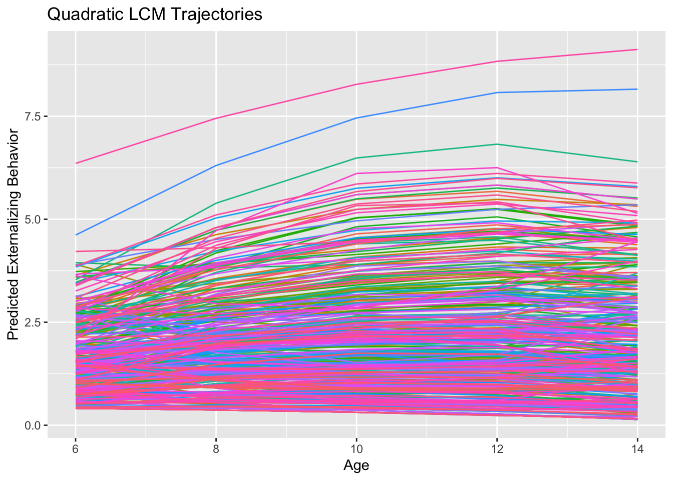
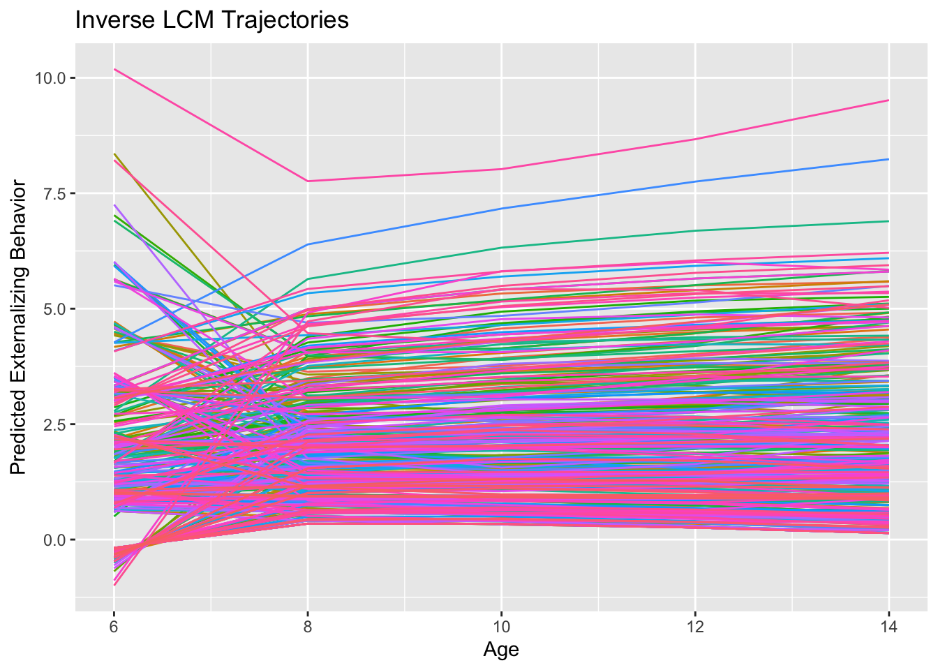
What should be visually apparent is that we get quite a few flips in the direction of curvature in the inverse compared to the quadratic model. Indeed the quadratic effect is negative (\(-0.015\)) and the inverse effect is positive (\(0.513\)). This sensitivity is likely another indication that curvature is really over-fitting noise in these data rather than reflecting some true non-linearity. Below are how to achieve this model with the MLM:
external.math.long$age_inv <- 1 - (external.math.long$age + 1)^(-1)

inv.mlm <- lmer(ext ~ 1 + age + age_inv + (1 + age + age_inv | id),
                na.action = na.omit,
                REML = TRUE,
                data = external.math.long,
                control = lmerControl(optimizer = "bobyqa",
                                      optCtrl = list(maxfun = 2e5)))

summary(inv.mlm, correlation = FALSE)
## Linear mixed model fit by REML. t-tests use Satterthwaite's method [
## lmerModLmerTest]
## Formula: ext ~ 1 + age + age_inv + (1 + age + age_inv | id)
## Data: external.math.long
## Control: lmerControl(optimizer = "bobyqa", optCtrl = list(maxfun = 2e+05))
##
## REML criterion at convergence: 5257.8
##
## Scaled residuals:
## Min 1Q Median 3Q Max
## -3.2607 -0.5446 -0.1801 0.4579 4.1099
##
## Random effects:
## Groups Name Variance Std.Dev. Corr
## id (Intercept) 0.83374 0.9131
## age 0.01219 0.1104 0.20
## age_inv 0.90843 0.9531 0.51 -0.17
## Residual 1.72232 1.3124
## Number of obs: 1357, groups: id, 405
##
## Fixed effects:
## Estimate Std. Error df t value Pr(>|t|)
## (Intercept) 1.56085 0.09081 319.40873 17.188 <2e-16 ***
## age 0.01432 0.02980 283.39325 0.480 0.6313
## age_inv 0.49152 0.21733 353.09910 2.262 0.0243 *
## ---
## Signif. codes: 0 '***' 0.001 '**' 0.01 '*' 0.05 '.' 0.1 ' ' 1anova(lin.mlm, inv.mlm)## Data: external.math.long
## Models:
## lin.mlm: ext ~ 1 + age + (1 + age | id)
## inv.mlm: ext ~ 1 + age + age_inv + (1 + age + age_inv | id)
## npar AIC BIC logLik deviance Chisq Df Pr(>Chisq)
## lin.mlm 6 5271.7 5303 -2629.9 5259.7
## inv.mlm 10 5266.9 5319 -2623.4 5246.9 12.825 4 0.01216 *
## ---
## Signif. codes: 0 '***' 0.001 '**' 0.01 '*' 0.05 '.' 0.1 ' ' 1and LCSM (note that the subtraction method gets a little messy for the slope loadings):
inv.lcsm <- "
            # Define Phantom Variables (p = phantom)
            pext6 =~ 1*ext6; ext6 ~ 0; ext6 ~~ ext6; pext6 ~~ 0*pext6
            pext8 =~ 1*ext8; ext8 ~ 0; ext8 ~~ ext8; pext8 ~~ 0*pext8
            pext10 =~ 1*ext10; ext10 ~ 0; ext10 ~~ ext10; pext10 ~~ 0*pext10
            pext12 =~ 1*ext12; ext12 ~ 0; ext12 ~~ ext12; pext12 ~~ 0*pext12
            pext14 =~ 1*ext14; ext14 ~ 0; ext14 ~~ ext14; pext14 ~~ 0*pext14

            # Regressions Between Adjacent Observations
            pext8 ~ 1*pext6
            pext10 ~ 1*pext8
            pext12 ~ 1*pext10
            pext14 ~ 1*pext12

            # Define Change Latent Variables (delta)
            delta21 =~ 1*pext8;  delta21 ~~ 0*delta21
            delta32 =~ 1*pext10; delta32 ~~ 0*delta32
            delta43 =~ 1*pext12; delta43 ~~ 0*delta43
            delta54 =~ 1*pext14; delta54 ~~ 0*delta54

            # Define Intercept and Slope
            int =~ 1*pext6
            slp =~ 2*delta21 + 2*delta32 + 2*delta43 + 2*delta54
            inv =~ (2/3)*delta21 + (2/15)*delta32 + (2/35)*delta43 + (1/56)*delta54

            int ~ 1
            slp ~ 1
            inv ~ 1

            int ~~ slp
            int ~~ inv
            slp ~~ slp
            slp ~~ inv
            inv ~~ inv
"

inv.lcsm.fit <- sem(inv.lcsm,
                    data = external.math,
                    estimator = "ML",
                    missing = "FIML")

summary(inv.lcsm.fit, fit.measures = FALSE, estimates = TRUE,
        standardize = TRUE, rsquare = FALSE)
## lavaan 0.6.13 ended normally after 64 iterations
##
## Estimator ML
## Optimization method NLMINB
## Number of model parameters 14
##
## Number of observations 405
## Number of missing patterns 21
##
## Model Test User Model:
##
## Test statistic 5.839
## Degrees of freedom 6
## P-value (Chi-square) 0.442
##
## Parameter Estimates:
##
## Standard errors Standard
## Information Observed
## Observed information based on Hessian
##
## Latent Variables:
## Estimate Std.Err z-value P(>|z|) Std.lv Std.all
## pext6 =~
## ext6 1.000 1.747 1.099
## pext8 =~
## ext8 1.000 1.397 0.739
## pext10 =~
## ext10 1.000 1.539 0.753
## pext12 =~
## ext12 1.000 1.655 0.786
## pext14 =~
## ext14 1.000 1.790 0.818
## delta21 =~
## pext8 1.000 1.140 1.140
## delta32 =~
## pext10 1.000 0.185 0.185
## delta43 =~
## pext12 1.000 0.166 0.166
## delta54 =~
## pext14 1.000 0.182 0.182
## int =~
## pext6 1.000 1.000 1.000
## slp =~
## delta21 2.000 0.225 0.225
## delta32 2.000 1.255 1.255
## delta43 2.000 1.301 1.301
## delta54 2.000 1.097 1.097
## inv =~
## delta21 0.667 1.141 1.141
## delta32 0.133 1.274 1.274
## delta43 0.057 0.566 0.566
## delta54 0.018 0.149 0.149
##
## Regressions:
## Estimate Std.Err z-value P(>|z|) Std.lv Std.all
## pext8 ~
## pext6 1.000 1.251 1.251
## pext10 ~
## pext8 1.000 0.908 0.908
## pext12 ~
## pext10 1.000 0.930 0.930
## pext14 ~
## pext12 1.000 0.925 0.925
##
## Covariances:
## Estimate Std.Err z-value P(>|z|) Std.lv Std.all
## int ~~
## slp 0.175 0.141 1.240 0.215 0.560 0.560
## inv -3.251 3.076 -1.057 0.290 -0.683 -0.683
## slp ~~
## inv -0.335 0.302 -1.109 0.267 -0.688 -0.688
##
## Intercepts:
## Estimate Std.Err z-value P(>|z|) Std.lv Std.all
## .ext6 0.000 0.000 0.000
## .ext8 0.000 0.000 0.000
## .ext10 0.000 0.000 0.000
## .ext12 0.000 0.000 0.000
## .ext14 0.000 0.000 0.000
## int 1.551 0.091 17.075 0.000 0.887 0.887
## slp 0.014 0.030 0.458 0.647 0.076 0.076
## inv 0.513 0.217 2.368 0.018 0.188 0.188
## .pext6 0.000 0.000 0.000
## .pext8 0.000 0.000 0.000
## .pext10 0.000 0.000 0.000
## .pext12 0.000 0.000 0.000
## .pext14 0.000 0.000 0.000
## .delta21 0.000 0.000 0.000
## .delta32 0.000 0.000 0.000
## .delta43 0.000 0.000 0.000
## .delta54 0.000 0.000 0.000
##
## Variances:
## Estimate Std.Err z-value P(>|z|) Std.lv Std.all
## .ext6 -0.523 1.838 -0.285 0.776 -0.523 -0.207
## .pext6 0.000 0.000 0.000
## .ext8 1.617 0.240 6.739 0.000 1.617 0.453
## .pext8 0.000 0.000 0.000
## .ext10 1.811 0.203 8.939 0.000 1.811 0.433
## .pext10 0.000 0.000 0.000
## .ext12 1.696 0.227 7.461 0.000 1.696 0.383
## .pext12 0.000 0.000 0.000
## .ext14 1.582 0.447 3.541 0.000 1.582 0.331
## .pext14 0.000 0.000 0.000
## .delta21 0.000 0.000 0.000
## .delta32 0.000 0.000 0.000
## .delta43 0.000 0.000 0.000
## .delta54 0.000 0.000 0.000
## slp 0.032 0.033 0.978 0.328 1.000 1.000
## inv 7.422 5.288 1.404 0.160 1.000 1.000
## int 3.052 1.850 1.650 0.099 1.000 1.000lavTestLRT(lin.lcsm.fit, inv.lcsm.fit)##
## Chi-Squared Difference Test
##
## Df AIC BIC Chisq Chisq diff RMSEA Df diff Pr(>Chisq)
## inv.lcsm.fit 6 5272.6 5328.6 5.8386
## lin.lcsm.fit 10 5278.2 5318.3 19.5065 13.668 0.077252 4 0.008434 **
## ---
## Signif. codes: 0 '***' 0.001 '**' 0.01 '*' 0.05 '.' 0.1 ' ' 1Piecewise Trajectories
If we do not think that a single polynomial function can sufficiently capture a complex trajectory, we might consider bolting two (or more) polynomial functions together using a piecewise approach. Here we will use the adversity data which covers \(8\) years of childhood (ages \(4-11\)). The simplest piecewise trajectory can be constructed two distinct linear pieces joined at a knot point. We need at least 3 time points to specify a line but the pieces can share a time point at the knot point. This means we need a minimum of \(5\) time points in order to fit even the simplest piecewise model. Note that with this minimum, the knot point is constrained to be at the middle time point, and the knot can never be placed at the first or last two time points because of the 3 time point requirement to estimate the linear slope. Note that as we discussed before, these time point requirements can be accomodated at the group level, and no one individual need be observed \(5\) or more times. Indeed this is the case here, where no individual is measured more than \(4\) times.
There are two general approaches for specifying piecewise models. The first, and more common, approach is the two-rate specification, where each effect can be interpreted in isolation like a regular linear model. We specify the two-rate LCM using the syntax below. Note that we code the factor loadings in such a way that the intercept is at the knot point (age 8).
two.rate <- "int  =~ 1*fmin4 + 1*fmin5 + 1*fmin6 + 1*fmin7 +
                     1*fmin8 + 1*fmin9 + 1*fmin10 + 1*fmin11
             slp1 =~ -3*fmin4 + -2*fmin5 + -1*fmin6 + 0*fmin7 +
                     0*fmin8 + 0*fmin9 + 0*fmin10 + 0*fmin11
             slp2 =~ 0*fmin4 + 0*fmin5 + 0*fmin6 + 0*fmin7 +
                     1*fmin8 + 2*fmin9 + 3*fmin10 + 4*fmin11
"

two.rate.fit <- growth(two.rate,
                       data = adversity,
                       estimator = "ML",
                       missing = "FIML")

summary(two.rate.fit, fit.measures = FALSE, estimates = TRUE,
        standardize = TRUE, rsquare = FALSE)
## lavaan 0.6.13 ended normally after 50 iterations
##
## Estimator ML
## Optimization method NLMINB
## Number of model parameters 17
##
## Number of observations 398
## Number of missing patterns 40
##
## Model Test User Model:
##
## Test statistic 35.322
## Degrees of freedom 27
## P-value (Chi-square) 0.131
##
## Parameter Estimates:
##
## Standard errors Standard
## Information Observed
## Observed information based on Hessian
##
## Latent Variables:
## Estimate Std.Err z-value P(>|z|) Std.lv Std.all
## int =~
## fmin4 1.000 0.886 0.888
## fmin5 1.000 0.886 0.942
## fmin6 1.000 0.886 0.824
## fmin7 1.000 0.886 0.761
## fmin8 1.000 0.886 0.706
## fmin9 1.000 0.886 0.720
## fmin10 1.000 0.886 0.739
## fmin11 1.000 0.886 0.661
## slp1 =~
## fmin4 -3.000 -0.985 -0.987
## fmin5 -2.000 -0.657 -0.698
## fmin6 -1.000 -0.328 -0.305
## fmin7 0.000 0.000 0.000
## fmin8 0.000 0.000 0.000
## fmin9 0.000 0.000 0.000
## fmin10 0.000 0.000 0.000
## fmin11 0.000 0.000 0.000
## slp2 =~
## fmin4 0.000 0.000 0.000
## fmin5 0.000 0.000 0.000
## fmin6 0.000 0.000 0.000
## fmin7 0.000 0.000 0.000
## fmin8 1.000 0.068 0.054
## fmin9 2.000 0.136 0.111
## fmin10 3.000 0.204 0.170
## fmin11 4.000 0.272 0.203
##
## Covariances:
## Estimate Std.Err z-value P(>|z|) Std.lv Std.all
## int ~~
## slp1 0.138 0.062 2.233 0.026 0.475 0.475
## slp2 0.027 0.045 0.602 0.547 0.449 0.449
## slp1 ~~
## slp2 0.011 0.019 0.548 0.584 0.475 0.475
##
## Intercepts:
## Estimate Std.Err z-value P(>|z|) Std.lv Std.all
## .fmin4 0.000 0.000 0.000
## .fmin5 0.000 0.000 0.000
## .fmin6 0.000 0.000 0.000
## .fmin7 0.000 0.000 0.000
## .fmin8 0.000 0.000 0.000
## .fmin9 0.000 0.000 0.000
## .fmin10 0.000 0.000 0.000
## .fmin11 0.000 0.000 0.000
## int 0.216 0.062 3.495 0.000 0.244 0.244
## slp1 0.079 0.029 2.741 0.006 0.239 0.239
## slp2 0.031 0.020 1.576 0.115 0.455 0.455
##
## Variances:
## Estimate Std.Err z-value P(>|z|) Std.lv Std.all
## .fmin4 0.069 0.388 0.178 0.859 0.069 0.069
## .fmin5 0.221 0.190 1.161 0.246 0.221 0.250
## .fmin6 0.539 0.103 5.231 0.000 0.539 0.466
## .fmin7 0.570 0.156 3.653 0.000 0.570 0.420
## .fmin8 0.731 0.129 5.671 0.000 0.731 0.464
## .fmin9 0.605 0.099 6.108 0.000 0.605 0.399
## .fmin10 0.450 0.123 3.664 0.000 0.450 0.312
## .fmin11 0.722 0.172 4.191 0.000 0.722 0.401
## int 0.786 0.151 5.215 0.000 1.000 1.000
## slp1 0.108 0.056 1.919 0.055 1.000 1.000
## slp2 0.005 0.019 0.240 0.810 1.000 1.000ggplot(data.frame(id=two.rate.fit@Data@case.idx[[1]],
lavPredict(two.rate.fit,type="ov")) %>%
pivot_longer(cols = starts_with("fmin"),
names_to = c(".value", "age"),
names_pattern = "(fmin)(.+)") %>%
dplyr::mutate(age = as.numeric(age)),
aes(x = age,
y = fmin,
group = id,
color = factor(id))) +
geom_line() +
labs(title = "2-Rate Piecewise LCM Trajectories",
x = "Age",
y = "Predicted Forceps Minor Microstructure") +
theme(legend.position = "none") 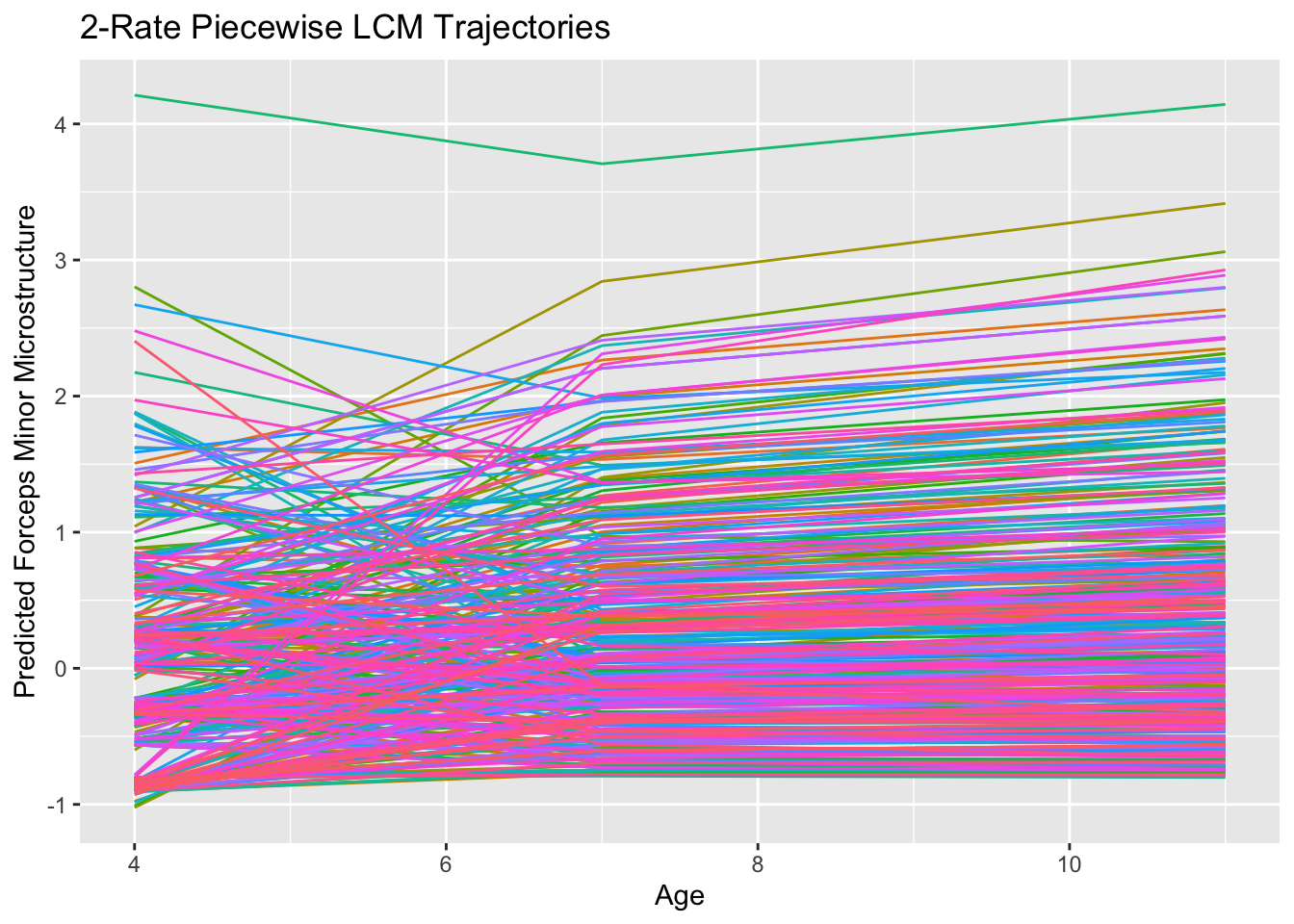
The second approach is the added-rate approach where the second slope is defined as the deflection from the original trajectory. We can see this approach below.
add.rate <- "int  =~ 1*fmin4 + 1*fmin5 + 1*fmin6 + 1*fmin7 +
                     1*fmin8 + 1*fmin9 + 1*fmin10 + 1*fmin11
             slp1 =~ -3*fmin4 + -2*fmin5 + -1*fmin6 + 0*fmin7 +
                     1*fmin8 + 2*fmin9 + 3*fmin10 + 4*fmin11
             slp2 =~ 0*fmin4 + 0*fmin5 + 0*fmin6 + 0*fmin7 +
                     1*fmin8 + 2*fmin9 + 3*fmin10 + 4*fmin11
"

add.rate.fit <- growth(add.rate,
                       data = adversity,
                       estimator = "ML",
                       missing = "FIML")

summary(add.rate.fit, fit.measures = FALSE, estimates = TRUE,
        standardize = TRUE, rsquare = FALSE)
## lavaan 0.6.13 ended normally after 44 iterations
##
## Estimator ML
## Optimization method NLMINB
## Number of model parameters 17
##
## Number of observations 398
## Number of missing patterns 40
##
## Model Test User Model:
##
## Test statistic 35.322
## Degrees of freedom 27
## P-value (Chi-square) 0.131
##
## Parameter Estimates:
##
## Standard errors Standard
## Information Observed
## Observed information based on Hessian
##
## Latent Variables:
## Estimate Std.Err z-value P(>|z|) Std.lv Std.all
## int =~
## fmin4 1.000 0.886 0.888
## fmin5 1.000 0.886 0.942
## fmin6 1.000 0.886 0.824
## fmin7 1.000 0.886 0.761
## fmin8 1.000 0.886 0.706
## fmin9 1.000 0.886 0.720
## fmin10 1.000 0.886 0.739
## fmin11 1.000 0.886 0.661
## slp1 =~
## fmin4 -3.000 -0.985 -0.987
## fmin5 -2.000 -0.657 -0.698
## fmin6 -1.000 -0.328 -0.305
## fmin7 0.000 0.000 0.000
## fmin8 1.000 0.328 0.262
## fmin9 2.000 0.657 0.533
## fmin10 3.000 0.985 0.821
## fmin11 4.000 1.314 0.980
## slp2 =~
## fmin4 0.000 0.000 0.000
## fmin5 0.000 0.000 0.000
## fmin6 0.000 0.000 0.000
## fmin7 0.000 0.000 0.000
## fmin8 1.000 0.302 0.241
## fmin9 2.000 0.604 0.491
## fmin10 3.000 0.906 0.755
## fmin11 4.000 1.209 0.901
##
## Covariances:
## Estimate Std.Err z-value P(>|z|) Std.lv Std.all
## int ~~
## slp1 0.138 0.062 2.233 0.026 0.475 0.475
## slp2 -0.111 0.101 -1.099 0.272 -0.415 -0.415
## slp1 ~~
## slp2 -0.097 0.067 -1.441 0.149 -0.980 -0.980
##
## Intercepts:
## Estimate Std.Err z-value P(>|z|) Std.lv Std.all
## .fmin4 0.000 0.000 0.000
## .fmin5 0.000 0.000 0.000
## .fmin6 0.000 0.000 0.000
## .fmin7 0.000 0.000 0.000
## .fmin8 0.000 0.000 0.000
## .fmin9 0.000 0.000 0.000
## .fmin10 0.000 0.000 0.000
## .fmin11 0.000 0.000 0.000
## int 0.216 0.062 3.495 0.000 0.244 0.244
## slp1 0.079 0.029 2.741 0.006 0.239 0.239
## slp2 -0.048 0.041 -1.150 0.250 -0.157 -0.157
##
## Variances:
## Estimate Std.Err z-value P(>|z|) Std.lv Std.all
## .fmin4 0.069 0.388 0.178 0.859 0.069 0.069
## .fmin5 0.221 0.190 1.161 0.246 0.221 0.250
## .fmin6 0.539 0.103 5.231 0.000 0.539 0.466
## .fmin7 0.570 0.156 3.653 0.000 0.570 0.420
## .fmin8 0.731 0.129 5.671 0.000 0.731 0.464
## .fmin9 0.605 0.099 6.108 0.000 0.605 0.399
## .fmin10 0.450 0.123 3.664 0.000 0.450 0.312
## .fmin11 0.722 0.172 4.191 0.000 0.722 0.401
## int 0.786 0.151 5.215 0.000 1.000 1.000
## slp1 0.108 0.056 1.919 0.055 1.000 1.000
## slp2 0.091 0.094 0.968 0.333 1.000 1.000Note that whichever approach we take, the models fit the data identically. This means that the choice between these two specifications should be guided by theoretical considerations of which type of effect you would prefer to interpret.
Of course, the models we have seen thus far in this section are the simplest linear-linear piecewise functions we can specify. We could even better specify these linear pieces with additional time points, or we could potentially increase the polynomial order of one or more of the pieces. This could be a great way to model nonlinear growth followed by a plateau for instance. Below, we demonstrate a quadratic-linear piecewise function that could capture this type of growth pattern. To identify this model, we can use trial-level data from the feedback.learning dataset source, with 4 trials specifying the quadratic initial piece, and the remaining trials specifying the second linear slope. Below we show the code to fit and visualize this model.
trials <- read.csv("data/trials.csv")

quad.rate <- "int =~ 1*trial.1 + 1*trial.2 + 1*trial.3 + 1*trial.4 +
                     1*trial.5 + 1*trial.6 + 1*trial.7
             slp1 =~ -3*trial.1 + -2*trial.2 + -1*trial.3 + 0*trial.4 +
                     0*trial.5 + 0*trial.6 + 0*trial.7
             quad =~ 9*trial.1 + 4*trial.2 + 1*trial.3 + 0*trial.4 +
                     0*trial.5 + 0*trial.6 + 0*trial.7
             slp2 =~ 0*trial.1 + 0*trial.2 + 0*trial.3 + 0*trial.4 +
                     1*trial.5 + 2*trial.6 + 3*trial.7

"

quad.rate.fit <- growth(quad.rate,
                       data = trials,
                       estimator = "ML",
                       missing = "FIML")

summary(quad.rate.fit, fit.measures = FALSE, estimates = TRUE,
        standardize = TRUE, rsquare = FALSE)
## lavaan 0.6.13 ended normally after 55 iterations
##
## Estimator ML
## Optimization method NLMINB
## Number of model parameters 21
##
## Number of observations 297
## Number of missing patterns 2
##
## Model Test User Model:
##
## Test statistic 46.778
## Degrees of freedom 14
## P-value (Chi-square) 0.000
##
## Parameter Estimates:
##
## Standard errors Standard
## Information Observed
## Observed information based on Hessian
##
## Latent Variables:
## Estimate Std.Err z-value P(>|z|) Std.lv Std.all
## int =~
## trial.1 1.000 0.900 0.904
## trial.2 1.000 0.900 0.866
## trial.3 1.000 0.900 0.821
## trial.4 1.000 0.900 0.830
## trial.5 1.000 0.900 0.819
## trial.6 1.000 0.900 0.780
## trial.7 1.000 0.900 0.718
## slp1 =~
## trial.1 -3.000 -0.846 -0.851
## trial.2 -2.000 -0.564 -0.543
## trial.3 -1.000 -0.282 -0.257
## trial.4 0.000 0.000 0.000
## trial.5 0.000 0.000 0.000
## trial.6 0.000 0.000 0.000
## trial.7 0.000 0.000 0.000
## quad =~
## trial.1 9.000 1.028 1.033
## trial.2 4.000 0.457 0.440
## trial.3 1.000 0.114 0.104
## trial.4 0.000 0.000 0.000
## trial.5 0.000 0.000 0.000
## trial.6 0.000 0.000 0.000
## trial.7 0.000 0.000 0.000
## slp2 =~
## trial.1 0.000 0.000 0.000
## trial.2 0.000 0.000 0.000
## trial.3 0.000 0.000 0.000
## trial.4 0.000 0.000 0.000
## trial.5 1.000 0.167 0.152
## trial.6 2.000 0.333 0.289
## trial.7 3.000 0.500 0.399
##
## Covariances:
## Estimate Std.Err z-value P(>|z|) Std.lv Std.all
## int ~~
## slp1 -0.067 0.061 -1.099 0.272 -0.264 -0.264
## quad -0.044 0.019 -2.275 0.023 -0.426 -0.426
## slp2 -0.001 0.024 -0.042 0.967 -0.007 -0.007
## slp1 ~~
## quad 0.029 0.027 1.060 0.289 0.895 0.895
## slp2 0.007 0.023 0.292 0.770 0.140 0.140
## quad ~~
## slp2 0.003 0.007 0.393 0.694 0.140 0.140
##
## Intercepts:
## Estimate Std.Err z-value P(>|z|) Std.lv Std.all
## .trial.1 0.000 0.000 0.000
## .trial.2 0.000 0.000 0.000
## .trial.3 0.000 0.000 0.000
## .trial.4 0.000 0.000 0.000
## .trial.5 0.000 0.000 0.000
## .trial.6 0.000 0.000 0.000
## .trial.7 0.000 0.000 0.000
## int 0.416 0.060 6.956 0.000 0.463 0.463
## slp1 -0.052 0.052 -1.006 0.314 -0.184 -0.184
## quad -0.065 0.017 -3.709 0.000 -0.566 -0.566
## slp2 0.164 0.020 8.193 0.000 0.983 0.983
##
## Variances:
## Estimate Std.Err z-value P(>|z|) Std.lv Std.all
## .trial.1 0.350 0.115 3.047 0.002 0.350 0.354
## .trial.2 0.285 0.036 7.954 0.000 0.285 0.265
## .trial.3 0.311 0.039 7.983 0.000 0.311 0.259
## .trial.4 0.365 0.049 7.506 0.000 0.365 0.311
## .trial.5 0.370 0.037 9.896 0.000 0.370 0.307
## .trial.6 0.414 0.044 9.298 0.000 0.414 0.311
## .trial.7 0.517 0.071 7.249 0.000 0.517 0.329
## int 0.810 0.091 8.930 0.000 1.000 1.000
## slp1 0.080 0.079 1.010 0.312 1.000 1.000
## quad 0.013 0.011 1.193 0.233 1.000 1.000
## slp2 0.028 0.012 2.334 0.020 1.000 1.000ggplot(data.frame(id=quad.rate.fit@Data@case.idx[[1]],
lavPredict(quad.rate.fit,type="ov")) %>%
pivot_longer(cols = starts_with("trial"),
names_to = c(".value", "num"),
names_pattern = "(trial).(.)") %>%
dplyr::mutate(num = as.numeric(num)),
aes(x = num,
y = trial,
group = id,
color = factor(id))) +
geom_line() +
labs(title = "Quadradic-Linear Piecewise LCM Trajectories",
x = "Age",
y = "Predicted Externalizing Behavior") +
theme(legend.position = "none") 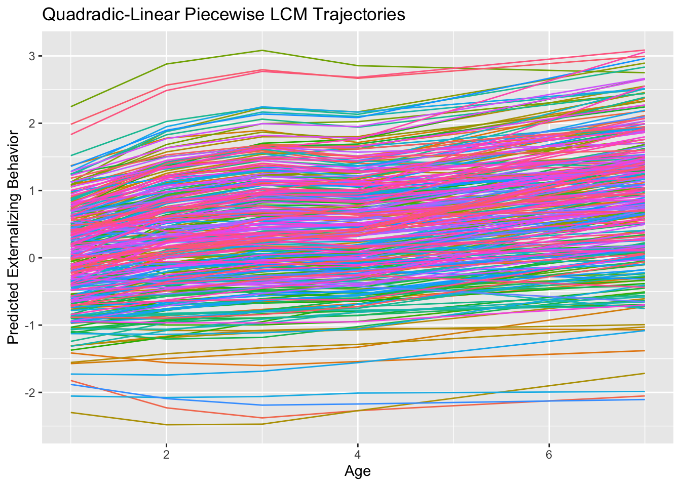
To fit piecewise models in the MLM, we simply create observed variables that correspond to the factor loadings we specified in the LCM code. Below we show how to generate these observed varaiables and the syntax to fit the two-rate version of the linear-linear model.
adversity.long <- adversity %>%
  pivot_longer(cols = starts_with("fmin"),
               names_to = c(".value", "age"),
               names_pattern = "(fmin)(.+)") %>%
  mutate(age = as.numeric(age),
         slp1 = ifelse(age > 7, 0, age - 7),
         slp2 = ifelse(age < 7, 0, age - 7),
         quad = ifelse(age > 7, 0, (age - 7)^2))

two.rate.mlm <- lmer(fmin ~ 1 + slp1 + slp2 + (1 + slp1 + slp2 | id),
                     na.action = na.omit,
                     REML = TRUE,
                     data = adversity.long,
                     control = lmerControl(optimizer = "bobyqa",
                                           optCtrl = list(maxfun = 2e5)))
summary(two.rate.mlm)
## Linear mixed model fit by REML. t-tests use Satterthwaite's method [
## lmerModLmerTest]
## Formula: fmin ~ 1 + slp1 + slp2 + (1 + slp1 + slp2 | id)
## Data: adversity.long
## Control: lmerControl(optimizer = "bobyqa", optCtrl = list(maxfun = 2e+05))
##
## REML criterion at convergence: 3565.7
##
## Scaled residuals:
## Min 1Q Median 3Q Max
## -3.2040 -0.5616 -0.2004 0.4489 3.9715
##
## Random effects:
## Groups Name Variance Std.Dev. Corr
## id (Intercept) 0.766249 0.8754
## slp1 0.020429 0.1429 1.00
## slp2 0.006305 0.0794 0.42 0.42
## Residual 0.635271 0.7970
## Number of obs: 1240, groups: id, 398
##
## Fixed effects:
## Estimate Std. Error df t value Pr(>|t|)
## (Intercept) 0.21114 0.06180 403.53944 3.417 0.000698 ***
## slp1 0.07239 0.02774 555.66344 2.610 0.009304 **
## slp2 0.03752 0.01968 335.58079 1.907 0.057417 .
## ---
## Signif. codes: 0 '***' 0.001 '**' 0.01 '*' 0.05 '.' 0.1 ' ' 1
##
## Correlation of Fixed Effects:
## (Intr) slp1
## slp1 0.676
## slp2 -0.450 -0.486
## optimizer (bobyqa) convergence code: 0 (OK)
## boundary (singular) fit: see help('isSingular')Fitting the piecewise model in the LCSM framework requires some additional work and unless we wish to include the dual-change effects, these models could be more-simply implemented as LCMs. This is due to a general complication in LCSMs if we wish to place the intercept anywhere except at the initial timepoint. If we look below at the Regressions Between Adjacent Observations section of the code below, we can see that for timepoints that come before the intercept (here before the knot point) we actually regression earlier timepoints on later timepoints. This reversal of the intuitive temporal order allows the LCSM to mimic the negative factor loadings in the LCM. Note also that the intercept timepoint (here pfmin7) appears twice, predicting the timepoint both before and after it. Finally, the loadings of the timepoints prior to the intercept load at a \(-1\) on the delta factors rather than a \(1\) as usual. The remainder of the model follows the conventions we are accustomed, but we comment below on the specific changes needed here.
two.rate.lcsm <- "
            # Define Phantom Variables (p = phantom)
            pfmin4 =~ 1*fmin4; fmin4 ~ 0; fmin4 ~~ fmin4; pfmin4 ~~ 0*fmin4
            pfmin5 =~ 1*fmin5; fmin5 ~ 0; fmin5 ~~ fmin5; pfmin5 ~~ 0*fmin5
            pfmin6 =~ 1*fmin6; fmin6 ~ 0; fmin6 ~~ fmin6; pfmin6 ~~ 0*fmin6
            pfmin7 =~ 1*fmin7; fmin7 ~ 0; fmin7 ~~ fmin7; pfmin7 ~~ 0*fmin7
            pfmin8 =~ 1*fmin8; fmin8 ~ 0; fmin8 ~~ fmin8; pfmin8 ~~ 0*fmin8
            pfmin9 =~ 1*fmin9; fmin9 ~ 0; fmin9 ~~ fmin9; pfmin9 ~~ 0*fmin9
            pfmin10 =~ 1*fmin10; fmin10 ~ 0; fmin10 ~~ fmin10; pfmin10 ~~ 0*fmin10
            pfmin11 =~ 1*fmin11; fmin11 ~ 0; fmin11 ~~ fmin11; pfmin11 ~~ 0*fmin11

            # Regressions Between Adjacent Observations
            pfmin4 ~ 1*pfmin5  # temporal order reversed before intercept
            pfmin5 ~ 1*pfmin6
            pfmin6 ~ 1*pfmin7
            pfmin8 ~ 1*pfmin7  # intercept time point appears twice
            pfmin9 ~ 1*pfmin8
            pfmin10 ~ 1*pfmin9
            pfmin11 ~ 1*pfmin10

            # Define Change Latent Variables (delta)
            # loadings prior to the intercept are negative
            delta21 =~ -1*pfmin4;  delta21 ~~ 0*delta21
            delta32 =~ -1*pfmin5;  delta32 ~~ 0*delta32
            delta43 =~ -1*pfmin6;  delta43 ~~ 0*delta43

            # loadings after the intercept are as usual
            delta54 =~ 1*pfmin8;  delta54 ~~ 0*delta54
            delta65 =~ 1*pfmin9;  delta65 ~~ 0*delta65
            delta76 =~ 1*pfmin10;  delta76 ~~ 0*delta76
            delta87 =~ 1*pfmin11;  delta87 ~~ 0*delta87

            # Define Intercept and Slope
            int  =~ 1*pfmin7
            slp1 =~ 1*delta21 + 1*delta32 + 1*delta43
            slp2 =~ 1*delta54 + 1*delta65 + 1*delta76 + 1*delta87

            int ~ 1; slp1 ~ 1; slp2 ~ 1

            slp1 ~~ slp1
            slp2 ~~ slp2
            int ~~ slp1 + slp2
            slp1 ~~ slp2
"
two.rate.lcsm.fit <- sem(two.rate.lcsm,
                         data = adversity,
                         estimator = "ML",
                         missing = "FIML")

summary(two.rate.lcsm.fit, fit.measures = FALSE, estimates = TRUE,
        standardize = TRUE, rsquare = FALSE)
## lavaan 0.6.13 ended normally after 50 iterations
##
## Estimator ML
## Optimization method NLMINB
## Number of model parameters 17
##
## Number of observations 398
## Number of missing patterns 40
##
## Model Test User Model:
##
## Test statistic 35.322
## Degrees of freedom 27
## P-value (Chi-square) 0.131
##
## Parameter Estimates:
##
## Standard errors Standard
## Information Observed
## Observed information based on Hessian
##
## Latent Variables:
## Estimate Std.Err z-value P(>|z|) Std.lv Std.all
## pfmin4 =~
## fmin4 1.000 0.963 0.965
## pfmin5 =~
## fmin5 1.000 0.815 0.866
## pfmin6 =~
## fmin6 1.000 0.786 0.731
## pfmin7 =~
## fmin7 1.000 0.886 0.761
## pfmin8 =~
## fmin8 1.000 0.919 0.732
## pfmin9 =~
## fmin9 1.000 0.955 0.776
## pfmin10 =~
## fmin10 1.000 0.995 0.829
## pfmin11 =~
## fmin11 1.000 1.038 0.774
## delta21 =~
## pfmin4 -1.000 -0.341 -0.341
## delta32 =~
## pfmin5 -1.000 -0.403 -0.403
## delta43 =~
## pfmin6 -1.000 -0.418 -0.418
## delta54 =~
## pfmin8 1.000 0.074 0.074
## delta65 =~
## pfmin9 1.000 0.071 0.071
## delta76 =~
## pfmin10 1.000 0.068 0.068
## delta87 =~
## pfmin11 1.000 0.066 0.066
## int =~
## pfmin7 1.000 1.000 1.000
## slp1 =~
## delta21 1.000 1.000 1.000
## delta32 1.000 1.000 1.000
## delta43 1.000 1.000 1.000
## slp2 =~
## delta54 1.000 1.000 1.000
## delta65 1.000 1.000 1.000
## delta76 1.000 1.000 1.000
## delta87 1.000 1.000 1.000
##
## Regressions:
## Estimate Std.Err z-value P(>|z|) Std.lv Std.all
## pfmin4 ~
## pfmin5 1.000 0.846 0.846
## pfmin5 ~
## pfmin6 1.000 0.964 0.964
## pfmin6 ~
## pfmin7 1.000 1.128 1.128
## pfmin8 ~
## pfmin7 1.000 0.965 0.965
## pfmin9 ~
## pfmin8 1.000 0.962 0.962
## pfmin10 ~
## pfmin9 1.000 0.960 0.960
## pfmin11 ~
## pfmin10 1.000 0.959 0.959
##
## Covariances:
## Estimate Std.Err z-value P(>|z|) Std.lv Std.all
## .pfmin4 ~~
## .fmin4 0.000 NaN NaN
## .pfmin5 ~~
## .fmin5 0.000 NaN NaN
## .pfmin6 ~~
## .fmin6 0.000 NaN NaN
## .pfmin7 ~~
## .fmin7 0.000 NaN NaN
## .pfmin8 ~~
## .fmin8 0.000 NaN NaN
## .pfmin9 ~~
## .fmin9 0.000 NaN NaN
## .pfmin10 ~~
## .fmin10 0.000 NaN NaN
## .pfmin11 ~~
## .fmin11 0.000 NaN NaN
## int ~~
## slp1 0.138 0.062 2.233 0.026 0.475 0.475
## slp2 0.027 0.045 0.602 0.547 0.449 0.449
## slp1 ~~
## slp2 0.011 0.019 0.548 0.584 0.475 0.475
##
## Intercepts:
## Estimate Std.Err z-value P(>|z|) Std.lv Std.all
## .fmin4 0.000 0.000 0.000
## .fmin5 0.000 0.000 0.000
## .fmin6 0.000 0.000 0.000
## .fmin7 0.000 0.000 0.000
## .fmin8 0.000 0.000 0.000
## .fmin9 0.000 0.000 0.000
## .fmin10 0.000 0.000 0.000
## .fmin11 0.000 0.000 0.000
## int 0.216 0.062 3.495 0.000 0.244 0.244
## slp1 0.079 0.029 2.741 0.006 0.239 0.239
## slp2 0.031 0.020 1.576 0.115 0.455 0.455
## .pfmin4 0.000 0.000 0.000
## .pfmin5 0.000 0.000 0.000
## .pfmin6 0.000 0.000 0.000
## .pfmin7 0.000 0.000 0.000
## .pfmin8 0.000 0.000 0.000
## .pfmin9 0.000 0.000 0.000
## .pfmin10 0.000 0.000 0.000
## .pfmin11 0.000 0.000 0.000
## .delta21 0.000 0.000 0.000
## .delta32 0.000 0.000 0.000
## .delta43 0.000 0.000 0.000
## .delta54 0.000 0.000 0.000
## .delta65 0.000 0.000 0.000
## .delta76 0.000 0.000 0.000
## .delta87 0.000 0.000 0.000
##
## Variances:
## Estimate Std.Err z-value P(>|z|) Std.lv Std.all
## .fmin4 0.069 0.388 0.178 0.859 0.069 0.069
## .fmin5 0.221 0.190 1.161 0.246 0.221 0.250
## .fmin6 0.539 0.103 5.231 0.000 0.539 0.466
## .fmin7 0.570 0.156 3.653 0.000 0.570 0.420
## .fmin8 0.731 0.129 5.671 0.000 0.731 0.464
## .fmin9 0.605 0.099 6.108 0.000 0.605 0.399
## .fmin10 0.450 0.123 3.664 0.000 0.450 0.312
## .fmin11 0.722 0.172 4.191 0.000 0.722 0.401
## .delta21 0.000 0.000 0.000
## .delta32 0.000 0.000 0.000
## .delta43 0.000 0.000 0.000
## .delta54 0.000 0.000 0.000
## .delta65 0.000 0.000 0.000
## .delta76 0.000 0.000 0.000
## .delta87 0.000 0.000 0.000
## slp1 0.108 0.056 1.919 0.055 1.000 1.000
## slp2 0.005 0.019 0.240 0.810 1.000 1.000
## .pfmin4 0.000 0.000 0.000
## .pfmin5 0.000 0.000 0.000
## .pfmin6 0.000 0.000 0.000
## .pfmin7 0.000 0.000 0.000
## .pfmin8 0.000 0.000 0.000
## .pfmin9 0.000 0.000 0.000
## .pfmin10 0.000 0.000 0.000
## .pfmin11 0.000 0.000 0.000
## int 0.786 0.151 5.215 0.000 1.000 1.000If we wish to include proportional change into this model, there is another additional oddity. For the beta parameters prior to the intercept, we actually create a cycle in our model (in technical terms the model is non-recursive), where the delta factor that a given phantom loads on is then regressed on that same phantom variable. The model remains identified, however, because the loading is fixed to \(-1\) while the proportional effect is freely estimated. The relevant syntax is below.
two.rate.prop.lcsm <- "
            # Define Phantom Variables (p = phantom)
            pfmin4 =~ 1*fmin4; fmin4 ~ 0; fmin4 ~~ fmin4; pfmin4 ~~ 0*fmin4
            pfmin5 =~ 1*fmin5; fmin5 ~ 0; fmin5 ~~ fmin5; pfmin5 ~~ 0*fmin5
            pfmin6 =~ 1*fmin6; fmin6 ~ 0; fmin6 ~~ fmin6; pfmin6 ~~ 0*fmin6
            pfmin7 =~ 1*fmin7; fmin7 ~ 0; fmin7 ~~ fmin7; pfmin7 ~~ 0*fmin7
            pfmin8 =~ 1*fmin8; fmin8 ~ 0; fmin8 ~~ fmin8; pfmin8 ~~ 0*fmin8
            pfmin9 =~ 1*fmin9; fmin9 ~ 0; fmin9 ~~ fmin9; pfmin9 ~~ 0*fmin9
            pfmin10 =~ 1*fmin10; fmin10 ~ 0; fmin10 ~~ fmin10; pfmin10 ~~ 0*fmin10
            pfmin11 =~ 1*fmin11; fmin11 ~ 0; fmin11 ~~ fmin11; pfmin11 ~~ 0*fmin11

            # Regressions Between Adjacent Observations
            pfmin4 ~ 1*pfmin5  # temporal order reversed before intercept
            pfmin5 ~ 1*pfmin6
            pfmin6 ~ 1*pfmin7
            pfmin8 ~ 1*pfmin7  # intercept time point appears twice
            pfmin9 ~ 1*pfmin8
            pfmin10 ~ 1*pfmin9
            pfmin11 ~ 1*pfmin10

            # Define Change Latent Variables (delta)
            # loadings prior to the intercept are negative
            delta21 =~ -1*pfmin4;  delta21 ~~ 0*delta21
            delta32 =~ -1*pfmin5;  delta32 ~~ 0*delta32
            delta43 =~ -1*pfmin6;  delta43 ~~ 0*delta43

            # loadings after the intercept are as usual
            delta54 =~ 1*pfmin8;  delta54 ~~ 0*delta54
            delta65 =~ 1*pfmin9;  delta65 ~~ 0*delta65
            delta76 =~ 1*pfmin10;  delta76 ~~ 0*delta76
            delta87 =~ 1*pfmin11;  delta87 ~~ 0*delta87

            # Define Proportional Change Regressions (beta = equality constraint)
            # Non-recursive Proportional Paths
            delta21 ~ beta*pfmin4
            delta32 ~ beta*pfmin5
            delta43 ~ beta*pfmin6

            # Standard Proportional Paths
            delta54 ~ beta*pfmin7
            delta65 ~ beta*pfmin8
            delta76 ~ beta*pfmin9
            delta87 ~ beta*pfmin10

            # Define Intercept and Slope
            int  =~ 1*pfmin7
            slp1 =~ 1*delta21 + 1*delta32 + 1*delta43
            slp2 =~ 1*delta54 + 1*delta65 + 1*delta76 + 1*delta87

            int ~ 1; slp1 ~ 1; slp2 ~ 1

            slp1 ~~ slp1
            slp2 ~~ slp2
            int ~~ slp1 + slp2
            slp1 ~~ slp2
"
two.rate.prop.lcsm.fit <- sem(two.rate.prop.lcsm,
                              data = adversity,
                              estimator = "ML",
                              missing = "FIML")

summary(two.rate.prop.lcsm.fit, fit.measures = FALSE, estimates = TRUE,
        standardize = TRUE, rsquare = FALSE)
## lavaan 0.6.13 ended normally after 773 iterations
##
## Estimator ML
## Optimization method NLMINB
## Number of model parameters 24
## Number of equality constraints 6
##
## Number of observations 398
## Number of missing patterns 40
##
## Model Test User Model:
##
## Test statistic 34.156
## Degrees of freedom 26
## P-value (Chi-square) 0.131
##
## Parameter Estimates:
##
## Standard errors Standard
## Information Observed
## Observed information based on Hessian
##
## Latent Variables:
## Estimate Std.Err z-value P(>|z|) Std.lv Std.all
## pfmin4 =~
## fmin4 1.000 0.763 0.741
## pfmin5 =~
## fmin5 1.000 0.747 0.800
## pfmin6 =~
## fmin6 1.000 0.741 0.705
## pfmin7 =~
## fmin7 1.000 0.881 0.747
## pfmin8 =~
## fmin8 1.000 0.893 0.720
## pfmin9 =~
## fmin9 1.000 0.919 0.757
## pfmin10 =~
## fmin10 1.000 0.974 0.820
## pfmin11 =~
## fmin11 1.000 1.070 0.779
## delta21 =~
## pfmin4 -1.000 -0.103 -0.103
## delta32 =~
## pfmin5 -1.000 -0.242 -0.242
## delta43 =~
## pfmin6 -1.000 -0.560 -0.560
## delta54 =~
## pfmin8 1.000 NA NA
## delta65 =~
## pfmin9 1.000 NA NA
## delta76 =~
## pfmin10 1.000 NA NA
## delta87 =~
## pfmin11 1.000 NA NA
## int =~
## pfmin7 1.000 1.000 1.000
## slp1 =~
## delta21 1.000 12.917 12.917
## delta32 1.000 5.618 5.618
## delta43 1.000 2.444 2.444
## slp2 =~
## delta54 1.000 NA NA
## delta65 1.000 NA NA
## delta76 1.000 NA NA
## delta87 1.000 NA NA
##
## Regressions:
## Estimate Std.Err z-value P(>|z|) Std.lv Std.all
## pfmin4 ~
## pfmin5 1.000 0.979 0.979
## pfmin5 ~
## pfmin6 1.000 0.992 0.992
## pfmin6 ~
## pfmin7 1.000 1.189 1.189
## pfmin8 ~
## pfmin7 1.000 0.986 0.986
## pfmin9 ~
## pfmin8 1.000 0.971 0.971
## pfmin10 ~
## pfmin9 1.000 0.944 0.944
## pfmin11 ~
## pfmin10 1.000 0.910 0.910
## delta21 ~
## pfmin4 (beta) 1.299 1.790 0.725 0.468 12.627 12.627
## delta32 ~
## pfmin5 (beta) 1.299 1.790 0.725 0.468 5.377 5.377
## delta43 ~
## pfmin6 (beta) 1.299 1.790 0.725 0.468 2.320 2.320
## delta54 ~
## pfmin7 (beta) 1.299 1.790 0.725 0.468 NA NA
## delta65 ~
## pfmin8 (beta) 1.299 1.790 0.725 0.468 NA NA
## delta76 ~
## pfmin9 (beta) 1.299 1.790 0.725 0.468 NA NA
## delta87 ~
## pfmin10 (beta) 1.299 1.790 0.725 0.468 NA NA
##
## Covariances:
## Estimate Std.Err z-value P(>|z|) Std.lv Std.all
## .pfmin4 ~~
## .fmin4 0.000 NaN NaN
## .pfmin5 ~~
## .fmin5 0.000 NaN NaN
## .pfmin6 ~~
## .fmin6 0.000 NaN NaN
## .pfmin7 ~~
## .fmin7 0.000 NaN NaN
## .pfmin8 ~~
## .fmin8 0.000 NaN NaN
## .pfmin9 ~~
## .fmin9 0.000 NaN NaN
## .pfmin10 ~~
## .fmin10 0.000 NaN NaN
## .pfmin11 ~~
## .fmin11 0.000 NaN NaN
## int ~~
## slp1 -0.550 0.925 -0.594 0.552 -0.615 -0.615
## slp2 -0.997 1.445 -0.690 0.490 -1.000 -1.000
## slp1 ~~
## slp2 0.713 2.177 0.327 0.743 0.621 0.621
##
## Intercepts:
## Estimate Std.Err z-value P(>|z|) Std.lv Std.all
## .fmin4 0.000 0.000 0.000
## .fmin5 0.000 0.000 0.000
## .fmin6 0.000 0.000 0.000
## .fmin7 0.000 0.000 0.000
## .fmin8 0.000 0.000 0.000
## .fmin9 0.000 0.000 0.000
## .fmin10 0.000 0.000 0.000
## .fmin11 0.000 0.000 0.000
## int 0.212 0.058 3.626 0.000 0.241 0.241
## slp1 -0.026 0.156 -0.165 0.869 -0.025 -0.025
## slp2 -0.265 0.410 -0.647 0.518 -0.234 -0.234
## .pfmin4 0.000 0.000 0.000
## .pfmin5 0.000 0.000 0.000
## .pfmin6 0.000 0.000 0.000
## .pfmin7 0.000 0.000 0.000
## .pfmin8 0.000 0.000 0.000
## .pfmin9 0.000 0.000 0.000
## .pfmin10 0.000 0.000 0.000
## .pfmin11 0.000 0.000 0.000
## .delta21 0.000 0.000 0.000
## .delta32 0.000 0.000 0.000
## .delta43 0.000 0.000 0.000
## .delta54 0.000 NA NA
## .delta65 0.000 NA NA
## .delta76 0.000 NA NA
## .delta87 0.000 NA NA
##
## Variances:
## Estimate Std.Err z-value P(>|z|) Std.lv Std.all
## .fmin4 0.478 0.284 1.685 0.092 0.478 0.451
## .fmin5 0.315 0.203 1.550 0.121 0.315 0.361
## .fmin6 0.555 0.112 4.945 0.000 0.555 0.502
## .fmin7 0.613 0.118 5.190 0.000 0.613 0.441
## .fmin8 0.743 0.136 5.478 0.000 0.743 0.482
## .fmin9 0.630 0.102 6.191 0.000 0.630 0.427
## .fmin10 0.463 0.121 3.840 0.000 0.463 0.328
## .fmin11 0.742 0.500 1.483 0.138 0.742 0.393
## .delta21 0.000 0.000 0.000
## .delta32 0.000 0.000 0.000
## .delta43 0.000 0.000 0.000
## .delta54 0.000 NA NA
## .delta65 0.000 NA NA
## .delta76 0.000 NA NA
## .delta87 0.000 NA NA
## slp1 1.029 2.469 0.417 0.677 1.000 1.000
## slp2 1.281 3.663 0.350 0.726 1.000 1.000
## .pfmin4 0.000 0.000 0.000
## .pfmin5 0.000 0.000 0.000
## .pfmin6 0.000 0.000 0.000
## .pfmin7 0.000 0.000 0.000
## .pfmin8 0.000 0.000 0.000
## .pfmin9 0.000 0.000 0.000
## .pfmin10 0.000 0.000 0.000
## .pfmin11 0.000 0.000 0.000
## int 0.776 0.114 6.816 0.000 1.000 1.000Nonlinear Trajectories
However, we sometimes need to move beyond well-defined polynomial models in order to capture the complexity of developmental change over time and consider truly nonlinear trajectories. This is most common in applications with dense observations within-person or that cover wide (i.e., decades) age-ranges between-person, although we can model true nonlinearities in standard applications with 4-6 timepoints. GAMMs will shine in the former case, while LCMs and LCSMs offer some options for the latter.
We can start with the GAMM syntax we are familiar with to specify a nonlinear trend across ages \(8-28\) in the feedback.learning data.
gamm <- gamm4(scale(modularity) ~ 1 + s(age),
              random = ~ (1 | id),
              data = feedback.learning)

gamtabs(gamm$gam, type = "html",
        pnames = c("Intercept"), snames = c("s(Age)"),
caption = "Modularity as a Function of Age")plot.gam(gamm$gam, se = TRUE, rug = TRUE, shade = TRUE,
xlab = "Age", ylab = "Fitted Modularity Values")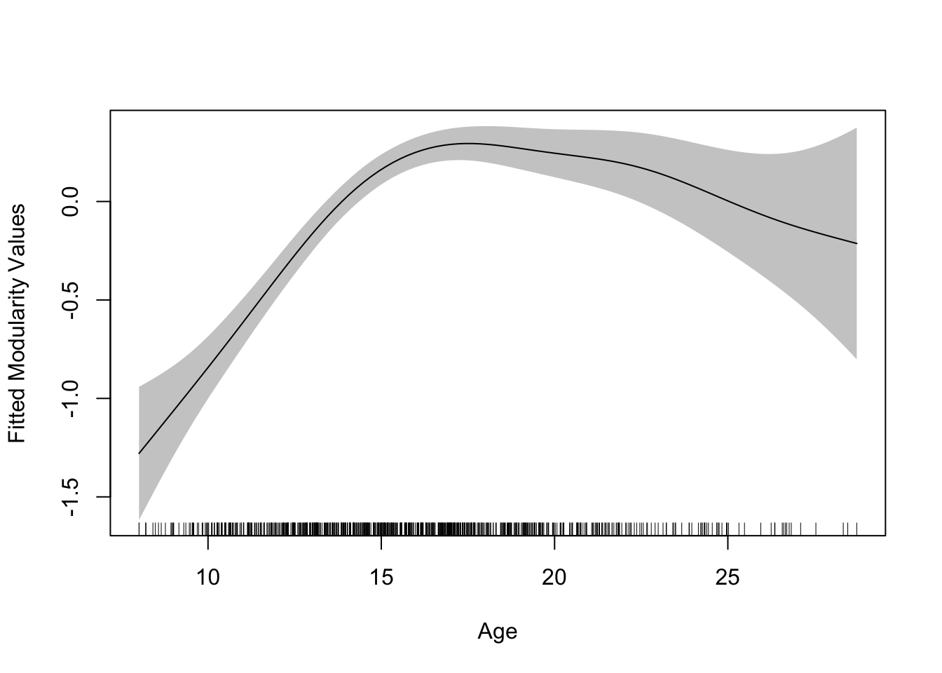
Nothing as changed about this model from what we have seen previously because the GAMM intrinsically captures non-linearities through the use of the splines. In principle, given the functional form that is revealed, these data might also be fit with a quadratic polynomial (indeed in McCormick et al., 2021, NeuroImage: see main analyses versus supplemental GAMMs as a sensitivity check). Indeed these models might be a nice tool for this purpose to check the reasonableness of the functional form specified in more restrictive polynomial models, even if we retain the polynomials for interpretability. With expanding age ranges, this type of sensitivity check becomes increasingly important, since the non-linearities of the GAMM are a better theoretical match for the complex patterns of growth across the lifespan. While deceptively simple in their implementation (indeed this is the exact same model we keep fitting), GAMMS are a powerful and flexible tool for fitting developmental trajectories.
The SEMs also allow for the inclusion of some nonlinear terms. Like the GAMM, we have already seen the most common nonlinearity through the proportional change parameter of the LCSM. We include the code and output for this model below but otherwise will not explore it further here.
executive.function <- read.csv("data/executive-function.csv", header = TRUE) %>%
  select(id, dlpfc1:dlpfc4)

proportional.lcsm <- "
               # Define Phantom Variables (p = phantom)
               pdlpfc1 =~ 1*dlpfc1; dlpfc1 ~ 0; dlpfc1 ~~ dlpfc1; pdlpfc1 ~~ 0*pdlpfc1
               pdlpfc2 =~ 1*dlpfc2; dlpfc2 ~ 0; dlpfc2 ~~ dlpfc2; pdlpfc2 ~~ 0*pdlpfc2
               pdlpfc3 =~ 1*dlpfc3; dlpfc3 ~ 0; dlpfc3 ~~ dlpfc3; pdlpfc3 ~~ 0*pdlpfc3
               pdlpfc4 =~ 1*dlpfc4; dlpfc4 ~ 0; dlpfc4 ~~ dlpfc4; pdlpfc4 ~~ 0*pdlpfc4

               # Regressions Between Adjacent Observations
               pdlpfc2 ~ 1*pdlpfc1
               pdlpfc3 ~ 1*pdlpfc2
               pdlpfc4 ~ 1*pdlpfc3

               # Define Change Latent Variables (delta)
               delta21 =~ 1*pdlpfc2; delta21 ~~ 0*delta21
               delta32 =~ 1*pdlpfc3; delta32 ~~ 0*delta32
               delta43 =~ 1*pdlpfc4; delta43 ~~ 0*delta43

               # Define Proportional Change Regressions (beta = equality constraint)
               delta21 ~ beta*pdlpfc1
               delta32 ~ beta*pdlpfc2
               delta43 ~ beta*pdlpfc3

               # Define Intercept and Slope
               int =~ 1*pdlpfc1
               slp =~ 1*delta21 + 1*delta32 + 1*delta43

               int ~ 1
               slp ~ 1

               int ~~ slp
               slp ~~ slp
"

lcsm.proportional <- sem(proportional.lcsm,
                         data = executive.function,
                         estimator = "ML",
                         missing = "FIML")

summary(lcsm.proportional)
## lavaan 0.6.13 ended normally after 32 iterations
##
## Estimator ML
## Optimization method NLMINB
## Number of model parameters 12
## Number of equality constraints 2
##
## Number of observations 342
## Number of missing patterns 8
##
## Model Test User Model:
##
## Test statistic 1.132
## Degrees of freedom 4
## P-value (Chi-square) 0.889
##
## Parameter Estimates:
##
## Standard errors Standard
## Information Observed
## Observed information based on Hessian
##
## Latent Variables:
## Estimate Std.Err z-value P(>|z|)
## pdlpfc1 =~
## dlpfc1 1.000
## pdlpfc2 =~
## dlpfc2 1.000
## pdlpfc3 =~
## dlpfc3 1.000
## pdlpfc4 =~
## dlpfc4 1.000
## delta21 =~
## pdlpfc2 1.000
## delta32 =~
## pdlpfc3 1.000
## delta43 =~
## pdlpfc4 1.000
## int =~
## pdlpfc1 1.000
## slp =~
## delta21 1.000
## delta32 1.000
## delta43 1.000
##
## Regressions:
## Estimate Std.Err z-value P(>|z|)
## pdlpfc2 ~
## pdlpfc1 1.000
## pdlpfc3 ~
## pdlpfc2 1.000
## pdlpfc4 ~
## pdlpfc3 1.000
## delta21 ~
## pdlpfc1 (beta) -0.090 0.276 -0.325 0.745
## delta32 ~
## pdlpfc2 (beta) -0.090 0.276 -0.325 0.745
## delta43 ~
## pdlpfc3 (beta) -0.090 0.276 -0.325 0.745
##
## Covariances:
## Estimate Std.Err z-value P(>|z|)
## int ~~
## slp -0.074 0.162 -0.457 0.647
##
## Intercepts:
## Estimate Std.Err z-value P(>|z|)
## .dlpfc1 0.000
## .dlpfc2 0.000
## .dlpfc3 0.000
## .dlpfc4 0.000
## int 0.540 0.054 9.994 0.000
## slp 0.179 0.183 0.981 0.326
## .pdlpfc1 0.000
## .pdlpfc2 0.000
## .pdlpfc3 0.000
## .pdlpfc4 0.000
## .delta21 0.000
## .delta32 0.000
## .delta43 0.000
##
## Variances:
## Estimate Std.Err z-value P(>|z|)
## .dlpfc1 0.208 0.102 2.043 0.041
## .pdlpfc1 0.000
## .dlpfc2 0.573 0.058 9.820 0.000
## .pdlpfc2 0.000
## .dlpfc3 0.577 0.060 9.570 0.000
## .pdlpfc3 0.000
## .dlpfc4 0.413 0.095 4.358 0.000
## .pdlpfc4 0.000
## .delta21 0.000
## .delta32 0.000
## .delta43 0.000
## slp 0.079 0.016 4.970 0.000
## int 0.796 0.115 6.925 0.000However, the LCM offers an unique opportunity to model non-linear trends by throwing back to its roots in confirmatory factor analysis. Instead of specifying factor loadings, as we have done up to this point, we can allow a subset of them to be freely-estimated. This means that equal change is estimated between each timepoint, growth can accelerate and decelerate across different increments. However, to identify the growth model, we have to set at least two of the factor loadings to pre-specified values (\(0\) and \(1\)) to set the scale for the other factor loadings. In general, there are two reasonable specifications. In the first, we set the first loading to \(0\) and the second to \(1\). This means that the other factor loadings are proportional to the amount of change that occurs between the first and second time point. We can see this specification below.
free.load1 <- "int   =~ 1*fmin4 + 1*fmin5 + 1*fmin6 + 1*fmin7 +
                        1*fmin8 + 1*fmin9 + 1*fmin10 + 1*fmin11
               basis =~ 0*fmin4 + 1*fmin5 + l3*fmin6 + l4*fmin7 +
                        l5*fmin8 + l6*fmin9 + l7*fmin10 + l8*fmin11
"

free.load1.fit <- growth(free.load1,
                         data = adversity,
                         estimator = "ML",
                         missing = "FIML")

summary(free.load1.fit, fit.measures = FALSE, estimates = TRUE,
        standardize = TRUE, rsquare = FALSE)
## lavaan 0.6.13 ended normally after 167 iterations
##
## Estimator ML
## Optimization method NLMINB
## Number of model parameters 19
##
## Number of observations 398
## Number of missing patterns 40
##
## Model Test User Model:
##
## Test statistic 22.185
## Degrees of freedom 25
## P-value (Chi-square) 0.625
##
## Parameter Estimates:
##
## Standard errors Standard
## Information Observed
## Observed information based on Hessian
##
## Latent Variables:
## Estimate Std.Err z-value P(>|z|) Std.lv Std.all
## int =~
## fmin4 1.000 0.600 0.591
## fmin5 1.000 0.600 0.649
## fmin6 1.000 0.600 0.549
## fmin7 1.000 0.600 0.517
## fmin8 1.000 0.600 0.468
## fmin9 1.000 0.600 0.511
## fmin10 1.000 0.600 0.531
## fmin11 1.000 0.600 0.431
## basis =~
## fmin4 0.000 0.000 0.000
## fmin5 1.000 0.043 0.046
## fmin6 (l3) 10.433 29.658 0.352 0.725 0.446 0.408
## fmin7 (l4) 10.668 29.930 0.356 0.722 0.456 0.393
## fmin8 (l5) 14.511 41.748 0.348 0.728 0.621 0.484
## fmin9 (l6) 10.347 28.955 0.357 0.721 0.443 0.377
## fmin10 (l7) 10.041 28.272 0.355 0.722 0.429 0.380
## fmin11 (l8) 22.493 65.845 0.342 0.733 0.962 0.691
##
## Covariances:
## Estimate Std.Err z-value P(>|z|) Std.lv Std.all
## int ~~
## basis 0.006 0.018 0.355 0.723 0.246 0.246
##
## Intercepts:
## Estimate Std.Err z-value P(>|z|) Std.lv Std.all
## .fmin4 0.000 0.000 0.000
## .fmin5 0.000 0.000 0.000
## .fmin6 0.000 0.000 0.000
## .fmin7 0.000 0.000 0.000
## .fmin8 0.000 0.000 0.000
## .fmin9 0.000 0.000 0.000
## .fmin10 0.000 0.000 0.000
## .fmin11 0.000 0.000 0.000
## int -0.011 0.068 -0.155 0.876 -0.018 -0.018
## basis 0.021 0.064 0.332 0.740 0.500 0.500
##
## Variances:
## Estimate Std.Err z-value P(>|z|) Std.lv Std.all
## .fmin4 0.671 0.134 5.021 0.000 0.671 0.651
## .fmin5 0.480 0.114 4.203 0.000 0.480 0.562
## .fmin6 0.505 0.101 5.008 0.000 0.505 0.422
## .fmin7 0.642 0.097 6.632 0.000 0.642 0.478
## .fmin8 0.716 0.146 4.911 0.000 0.716 0.436
## .fmin9 0.691 0.094 7.340 0.000 0.691 0.502
## .fmin10 0.606 0.107 5.656 0.000 0.606 0.475
## .fmin11 0.368 0.215 1.712 0.087 0.368 0.190
## int 0.360 0.109 3.292 0.001 1.000 1.000
## basis 0.002 0.011 0.167 0.867 1.000 1.000Here we label the freely-estimated factor loadings for convenient reference. We also specify the second factor as a basis (or sometimes “shape”) rather than a “slope” factor to reflect the non-linearity inherent in this model. When we examine the model results, we can see a pretty striking pattern of factor loadings. The third loading (l3) is \(10.43\), which suggests that more than \(9\) times the amount of change occurs between the second and third timepoints as does between the first two (remember we take the difference between adjacent loadings). However, l4 suggests that then there is a sharp deceleration in growth between the next timepoints. At l6, we can see that the factor loading actuall decreases, which is how this model fits a negative trend between adjacent timepoints. Finally, l8 suggests a large increase at the final timepoint, reversing the earlier decreases. One thing to highlight is the increase in complexity just in describing the factor loadings and interpreting adjacent timepoints that do not follow some monotonic trend. Like many non-linear models, visualization of the model-implied trajectories is key for interpreting the effects. We can do so below.
ggplot(data.frame(id=free.load1.fit@Data@case.idx[[1]],
                           lavPredict(free.load1.fit,type="ov")) %>%
                  pivot_longer(cols = starts_with("fmin"),
                               names_to = c(".value", "age"),
                               names_pattern = "(fmin)(.+)") %>%
                  dplyr::mutate(age = as.numeric(age)),
                aes(x = age,
                    y = fmin,
                    group = id,
                    color = factor(id))) +
  geom_line() +
  labs(title = "Free-loading Model 1 Trajectories",
       x = "Age",
       y = "Predicted Forceps Minor Microstructure") +
theme(legend.position = "none") 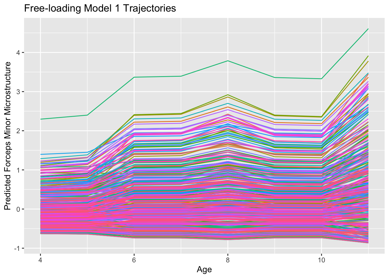
Here we can see the power, and danger, of these free-loading model. Like a GAMM, we can have complex, localized change, with reversals and highly variable slopes. However, in looking at the first couple of timepoints, we have to wonder if we are overfitting noise in the data when some simpler functional form would (e.g., a line) would describe this trend in a more replicable/generalizable way. Very often, these free-loading models will fit the data better than many alternatives we have discussed elsewhere in this primer, but then be very sample-depenedent in an unsatisfying fashion. Like with the GAMM, one potential use for this model is as a sensitivity check for a more-constrained LCM to ensure we are not completely botching the functional form.
We can refit this model using a different specification where we set the first loading to \(0\) and the last loading to \(1\). This scales the estimated loadings to be proportions of the total growth realized by that point. We can see this model below.
free.load2 <- "int   =~ 1*fmin4 + 1*fmin5 + 1*fmin6 + 1*fmin7 +
                        1*fmin8 + 1*fmin9 + 1*fmin10 + 1*fmin11
               basis =~ 0*fmin4 + l2*fmin5 + l3*fmin6 + l4*fmin7 +
                        l5*fmin8 + l6*fmin9 + l7*fmin10 + 1*fmin11
"

free.load2.fit <- growth(free.load2,
                         data = adversity,
                         estimator = "ML",
                         missing = "FIML")

summary(free.load2.fit, fit.measures = FALSE, estimates = TRUE,
        standardize = TRUE, rsquare = FALSE)
## lavaan 0.6.13 ended normally after 50 iterations
##
## Estimator ML
## Optimization method NLMINB
## Number of model parameters 19
##
## Number of observations 398
## Number of missing patterns 40
##
## Model Test User Model:
##
## Test statistic 22.185
## Degrees of freedom 25
## P-value (Chi-square) 0.625
##
## Parameter Estimates:
##
## Standard errors Standard
## Information Observed
## Observed information based on Hessian
##
## Latent Variables:
## Estimate Std.Err z-value P(>|z|) Std.lv Std.all
## int =~
## fmin4 1.000 0.600 0.591
## fmin5 1.000 0.600 0.649
## fmin6 1.000 0.600 0.549
## fmin7 1.000 0.600 0.517
## fmin8 1.000 0.600 0.468
## fmin9 1.000 0.600 0.511
## fmin10 1.000 0.600 0.531
## fmin11 1.000 0.600 0.431
## basis =~
## fmin4 0.000 0.000 0.000
## fmin5 (l2) 0.044 0.130 0.342 0.733 0.043 0.046
## fmin6 (l3) 0.464 0.117 3.962 0.000 0.446 0.408
## fmin7 (l4) 0.474 0.118 4.036 0.000 0.456 0.393
## fmin8 (l5) 0.645 0.141 4.564 0.000 0.621 0.484
## fmin9 (l6) 0.460 0.121 3.800 0.000 0.443 0.377
## fmin10 (l7) 0.446 0.148 3.024 0.002 0.429 0.380
## fmin11 1.000 0.962 0.691
##
## Covariances:
## Estimate Std.Err z-value P(>|z|) Std.lv Std.all
## int ~~
## basis 0.142 0.168 0.842 0.400 0.246 0.246
##
## Intercepts:
## Estimate Std.Err z-value P(>|z|) Std.lv Std.all
## .fmin4 0.000 0.000 0.000
## .fmin5 0.000 0.000 0.000
## .fmin6 0.000 0.000 0.000
## .fmin7 0.000 0.000 0.000
## .fmin8 0.000 0.000 0.000
## .fmin9 0.000 0.000 0.000
## .fmin10 0.000 0.000 0.000
## .fmin11 0.000 0.000 0.000
## int -0.011 0.068 -0.155 0.876 -0.018 -0.018
## basis 0.481 0.102 4.729 0.000 0.500 0.500
##
## Variances:
## Estimate Std.Err z-value P(>|z|) Std.lv Std.all
## .fmin4 0.671 0.134 5.021 0.000 0.671 0.651
## .fmin5 0.480 0.114 4.203 0.000 0.480 0.562
## .fmin6 0.505 0.101 5.008 0.000 0.505 0.422
## .fmin7 0.642 0.097 6.632 0.000 0.642 0.478
## .fmin8 0.716 0.146 4.911 0.000 0.716 0.436
## .fmin9 0.691 0.094 7.340 0.000 0.691 0.502
## .fmin10 0.606 0.107 5.656 0.000 0.606 0.475
## .fmin11 0.368 0.215 1.712 0.087 0.368 0.190
## int 0.360 0.109 3.292 0.001 1.000 1.000
## basis 0.925 0.385 2.404 0.016 1.000 1.000We can see that the loadings are now all less than \(1\) but that they follow the same pattern as in the model (which they should, as they are identically-fitting models). However, now the loadings are expressed as percentages of the total change that occurs between the first and final timepoint. Note one odd thing is that when a trajectory follows a parabolic shape, we can get loadings about \(1\) reflecting \(>100%\) of the overall change has occurred by that time point. Nothing is wrong, per se, with that interpretation, but given the oddness of language it evokes, the first specification is by far the more common.
Fixed and Random Effects
Before we move on, we want to highlight the distinction we make between fixed and random effects when we talk about the limitations of the functional form with respect to the number of repeated measures, per person. The oft-repeated mantra is that you need \(3\) timepoints for a line, \(4\) for a quadratic, and so on ad infinitum. But, on the other hand, we can fit a highly complex non-linear developmental trajectory to data where each individual contributes at most \(2\) timepoints. How do we reconcile these two things? Well it has to do with whether we treat the effect in question as fixed or random. When we treat a parameter as fixed, we obtain a single value that describes all indiviudals in our sample (barring pesky things like interactions), but when we treat an effect as random, we also model individual differences in that “fixed” parameter (note that we estimate a single variance per random effect, not individual effects, but that’s a longer discussion and we can calculate individual effects with some well-developed methods). So to estimate these individually-varying random effects, we need more repeated measures within-person. However, we can still estimate an overall fixed effect trajectory that takes advantage of greater timepoints between individuals than exist for any given individual. This is how we might estimate a GAMM with some highly complex surface, even though we could never estimate a random effect for any individual since they only contribute up to two observations.
We can demonstrate this with our feedback.learning data where we can model both the effect of wave, which is a fully within-person measure, as well as linear and quadratic age. These latter two effects are specified as fixed effects because while age between-person ranges from \(8 - 29\), no one person contributes more than \(3\) time points, so the quadratic random effect would not be estimable. However, we can estimate a random effect of wave. We can see these effects below. This distinction highlights some of the advantages of having measurement timing heterogeneity for estimating more complex effect than one could do with single-cohort data with fully consistent assessment schedules.
feedback.learning <- read.csv("data/feedback-learning.csv") %>%
  select(id, wave, age, modularity, learning.rate)

fixrand <- lmer(scale(modularity) ~ 1 + wave + age + I(age^2) +
                  (1 + wave | id),
                na.action = na.omit,
                REML = TRUE,
                data = feedback.learning)

summary(fixrand, correlation = FALSE)
## Linear mixed model fit by REML. t-tests use Satterthwaite's method [
## lmerModLmerTest]
## Formula: scale(modularity) ~ 1 + wave + age + I(age^2) + (1 + wave | id)
## Data: feedback.learning
##
## REML criterion at convergence: 1852.3
##
## Scaled residuals:
## Min 1Q Median 3Q Max
## -3.04443 -0.56388 0.00211 0.54870 2.45150
##
## Random effects:
## Groups Name Variance Std.Dev. Corr
## id (Intercept) 0.42472 0.6517
## wave 0.01452 0.1205 0.00
## Residual 0.36813 0.6067
## Number of obs: 754, groups: id, 297
##
## Fixed effects:
## Estimate Std. Error df t value Pr(>|t|)
## (Intercept) -4.653017 0.450546 424.620702 -10.328 < 2e-16 ***
## wave -0.021516 0.038502 499.253403 -0.559 0.577
## age 0.517778 0.055054 451.217127 9.405 < 2e-16 ***
## I(age^2) -0.013251 0.001576 467.828242 -8.410 4.99e-16 ***
## ---
## Signif. codes: 0 '***' 0.001 '**' 0.01 '*' 0.05 '.' 0.1 ' ' 1